|
|
Home | Switchboard | Unix Administration | Red Hat | TCP/IP Networks | Neoliberalism | Toxic Managers |
| (slightly skeptical) Educational society promoting "Back to basics" movement against IT overcomplexity and bastardization of classic Unix | |||||||
|
|
"Languages come and go,
but algorithms stand the test of time"
"An algorithm must be seen to be believed."
Donald Knuth
The quality of CS education is by-and-large determined by the knowledge of algorithms as well as OS and compilers internals (which utilize several rather complex algorithms). Unfortunately since late 70th the USA the level of CS education gradually deteriorated to the extent that even bright students graduate with rather superficial knowledge of those topics. As such they are second class programmers no matter how hard they try to learn the latest fancy OO-oriented language.
Why should you want to know more about algorithms? There are a number of possible reasons:
Those formulas mean that for sorting a small number of items simpler algorithms (or shellsort) are better than quicksort and for sorting large number of items mergesort is better as it can utilize natural orderness of the data ( can benefit from the fact that most "real" files are partially sorted; quicksort does not take into account this property; moreover it demonstrates worst case behavior on some nearly sorted files). Partially ordered files probably represent the most important in practice case of sorting that is often overlooked in superficial books. Often sorting is initiated just to put a few new records in proper place of the already sorted file.
BTW this is a good litmus test of a quality of any book that covers sorting;
if a book does not provide this information you might try to find another.
|
|
For all these reasons it is useful to have a broad familiarity with a range of algorithms, and to understand what types of problems they can help to solve. This is especially important for open source developers. Algorithms are intrinsically connected with data structures because data structures are dreaming to become elegant algorithms the same way ordinary people are dreaming about Hollywood actors ;-)
I would like to note that the value of browsing the WEB in search of algorithms is somewhat questionable :-). One probably will be much better off buying Donald Knuth's TAOCP and ... disconnecting from the Internet for a couple of months. Internet contains way too much noise that suppress useful signal... This is especially true about algorithms.
Note: MIX assembler is not very essential :-). Actually it represent class of computers which became obsolete even before the first volume Knuth book was published (with the release of IBM 360 which took world by storm). You can use Intel assembler if you wish. I used to teach TAOCP on mainframes and IBM assembler was pretty much OK. Knuth probably would be better off using a derivative of S/360 architecture and assembler from the very beginning ;-).Later he updated MIX to MMIX with a new instruction set for use in future volumes, but still existing three volumes use an old one. There are pages on Internet that have them rewritten in IBM 260 or other more modern instruction set.
An extremely important and often overlooked class of algorithms are compiler algorithms (lex analysis, parsing and code generation). They actually represent a very efficient paradigm for solving wide class of tasks similar to compilation of the program. For example complex conversions from one format to another. Also any complex program usually has its own command language and knowledge of compiler algorithms can prevent authors from making typical for amateurs blunders (which are common in open source software). In a way Greenspun's tenth rule - Wikipedia, the free encyclopedia
Any sufficiently complicated C or Fortran program contains an ad hoc, informally-specified, bug-ridden, slow implementation of half of Common Lisp.
can be reformulated to:
Any sufficiently complicated contains an ad hoc, informally-specified, bug-ridden, slow implementation of half of a typical programming language interpreter.
Many authors writing about algorithms try to hide their lack of competence with abuse of mathematical symbolic. Excessive use of mathematics in presentation of algorithms is often counterproductive (verification fiasco can serve as a warning for all future generation; it buried such talented authors as E. Dijkstra, David Gries and many others). Please remember Famous Donald Knuth's citation about correctness proofs:
On March 22, 1977, as I was drafting Section 7.1 of The Art of Computer Programming, I read four papers by Peter van Emde Boas that turned out to be more appropriate for Chapter 8 than Chapter 7. I wrote a five-page memo entitled ``Notes on the van Emde Boas construction of priority deques: An instructive use of recursion,'' and sent it to Peter on March 29 (with copies also to Bob Tarjan and John Hopcroft). The final sentence was this: ``Beware of bugs in the above code; I have only proved it correct, not tried it.''
See also Softpanorama Computer Books Reviews / Algorithms
Dr. Nikolai Bezroukov
P.S: In order to save the bandwidth for humans (as opposed to robots ;-), previous years of Old News section were converted into separate pages.
|
|
Switchboard | ||||
| Latest | |||||
| Past week | |||||
| Past month | |||||
| 2005 | 2004 | 2003 | 2002 | 2001 | 2000 | 1999 |
Nov 21, 2019 | perlmonks.org
This code was written as a solution to the problem posed in Search for identical substrings . As best I can tell it runs about 3 million times faster than the original code.
The code reads a series of strings and searches them for the longest substring between any pair of strings. In the original problem there were 300 strings about 3K long each. A test set comprising 6 strings was used to test the code with the result given below.
Someone with Perl module creation and publication experience could wrap this up and publish it if they wish.
use strict;
use warnings;
use Time::HiRes;
use List::Util qw(min max);

my $allLCS = 1;
my $subStrSize = 8; # Determines minimum match length. Should be a power of 2
# and less than half the minimum interesting match length. The larger this value
# the faster the search runs.

if (@ARGV != 1)
    {
    print "Finds longest matching substring between any pair of test strings\n";
    print "the given file. Pairs of lines are expected with the first of a\n";
    print "pair being the string name and the second the test string.";
    exit (1);
    }

# Read in the strings
my @strings;
while ()
  {
  chomp;
  my $strName = $_;
  $_ = ;
  chomp;
  push @strings, [$strName, $_];
  }

my $lastStr = @strings - 1;
my @bestMatches = [(0, 0, 0, 0, 0)]; # Best match details
my $longest = 0; # Best match length so far (unexpanded)

my $startTime = [Time::HiRes::gettimeofday ()];

# Do the search
for (0..$lastStr)
  {
  my $curStr = $_;
  my @subStrs;
  my $source = $strings[$curStr][1];
  my $sourceName = $strings[$curStr][0];

  for (my $i = 0; $i  0;
        push @localBests, [@test] if $dm >= 0;
        $offset = $test[3] + $test[4];

        next if $test[4]  0;
        push @bestMatches, [@test];
        }
        continue {++$offset;}
      }

    next if ! $allLCS;

    if (! @localBests)
      {
      print "Didn't find LCS for $sourceName and $targetName\n";
      next;
      }

    for (@localBests)
      {
      my @curr = @$_;
      printf "%03d:%03d L[%4d] (%4d %4d)\n",
        $curr[0], $curr[1], $curr[4], $curr[2], $curr[3];
      }
    }
  }

print "Completed in " . Time::HiRes::tv_interval ($startTime) . "\n";
for (@bestMatches)
  {
  my @curr = @$_;
  printf "Best match: %s - %s. %d characters starting at %d and %d.\n",
    $strings[$curr[0]][0], $strings[$curr[1]][0], $curr[4], $curr[2], $curr[3];
  }


sub expandMatch
{
my ($index1, $index2, $str1Start, $str2Start, $matchLen) = @_;
my $maxMatch = max (0, min ($str1Start, $subStrSize + 10, $str2Start));
my $matchStr1 = substr ($strings[$index1][1], $str1Start - $maxMatch, $maxMatch);
my $matchStr2 = substr ($strings[$index2][1], $str2Start - $maxMatch, $maxMatch);

($matchStr1 ^ $matchStr2) =~ /\0*$/;
my $adj = $+[0] - $-[0];
$matchLen += $adj;
$str1Start -= $adj;
$str2Start -= $adj;

return ($index1, $index2, $str1Start, $str2Start, $matchLen);
}
Output using bioMan 's six string sample:
Completed in 0.010486 Best match: >string 1 - >string 3 . 1271 characters starting at 82 an + d 82. [download]
Oct 13, 2019 | www.quora.com
Eugene Miya , A friend/colleague. Sometimes driver. Other shared experiences. Updated Mar 22 2017 · Author has 11.2k answers and 7.9m answer views
He mostly writes in C today.
I can assure you he at least knows about Python. Guido's office at Dropbox is 1 -- 2 blocks by a backdoor gate from Don's house.
I would tend to doubt that he would use R (I've used S before as one of my stat packages). Don would probably write something for himself.
Don is not big on functional languages, so I would doubt either Haskell (sorry Paul) or LISP (but McCarthy lived just around the corner from Don; I used to drive him to meetings; actually, I've driven all 3 of us to meetings, and he got his wife an electric version of my car based on riding in my car (score one for friend's choices)). He does use emacs and he does write MLISP macros, but he believes in being closer to the hardware which is why he sticks with MMIX (and MIX) in his books.
Don't discount him learning the machine language of a given architecture.
I'm having dinner with Don and Jill and a dozen other mutual friends in 3 weeks or so (our quarterly dinner). I can ask him then, if I remember (either a calendar entry or at job). I try not to bother him with things like this. Don is well connected to the hacker community
Don's name was brought up at an undergrad architecture seminar today, but Don was not in the audience (an amazing audience; I took a photo for the collection of architects and other computer scientists in the audience (Hennessey and Patterson were talking)). I came close to biking by his house on my way back home.
We do have a mutual friend (actually, I introduced Don to my biology friend at Don's request) who arrives next week, and Don is my wine drinking proxy. So there is a chance I may see him sooner.
Steven de Rooij , Theoretical computer scientist Answered Mar 9, 2017 · Author has 4.6k answers and 7.7m answer views
Nice question :-)
Don Knuth would want to use something that’s low level, because details matter . So no Haskell; LISP is borderline. Perhaps if the Lisp machine ever had become a thing.
He’d want something with well-defined and simple semantics, so definitely no R. Python also contains quite a few strange ad hoc rules, especially in its OO and lambda features. Yes Python is easy to learn and it looks pretty, but Don doesn’t care about superficialities like that. He’d want a language whose version number is converging to a mathematical constant, which is also not in favor of R or Python.
What remains is C. Out of the five languages listed, my guess is Don would pick that one. But actually, his own old choice of Pascal suits him even better. I don’t think any languages have been invented since was written that score higher on the Knuthometer than Knuth’s own original pick.
And yes, I feel that this is actually a conclusion that bears some thinking about. 24.1k views ·
Dan Allen , I've been programming for 34 years now. Still not finished. Answered Mar 9, 2017 · Author has 4.5k answers and 1.8m answer views
In The Art of Computer Programming I think he'd do exactly what he did. He'd invent his own architecture and implement programs in an assembly language targeting that theoretical machine.
He did that for a reason because he wanted to reveal the detail of algorithms at the lowest level of detail which is machine level.
He didn't use any available languages at the time and I don't see why that would suit his purpose now. All the languages above are too high-level for his purposes.
Sep 07, 2019 | archive.computerhistory.org
Knuth: Yeah. That's absolutely true. I've got to get another thought out of my mind though. That is, early on in the TeX project I also had to do programming of a completely different type. I told you last week that this was my first real exercise in structured programming, which was one of Dijkstra's huge... That's one of the few breakthroughs in the history of computer science, in a way. He was actually responsible for maybe two of the ten that I know.
So I'm doing structured programming as I'm writing TeX. I'm trying to do it right, the way I should've been writing programs in the 60s. Then I also got this typesetting machine, which had, inside of it, a tiny 8080 chip or something. I'm not sure exactly. It was a Zilog, or some very early Intel chip. Way before the 386s. A little computer with 8-bit registers and a small number of things it could do. I had to write my own assembly language for this, because the existing software for writing programs for this little micro thing were so bad. I had to write actually thousands of lines of code for this, in order to control the typesetting. Inside the machine I had to control a stepper motor, and I had to accelerate it.
Every so often I had to give another [command] saying, "Okay, now take a step," and then continue downloading a font from the mainframe.
I had six levels of interrupts in this program. I remember talking to you at this time, saying, "Ed, I'm programming in assembly language for an 8-bit computer," and you said "Yeah, you've been doing the same thing and it's fun again."
You know, you'll remember. We'll undoubtedly talk more about that when I have my turn interviewing you in a week or so. This is another aspect of programming: that you also feel that you're in control and that there's not a black box separating you. It's not only the power, but it's the knowledge of what's going on; that nobody's hiding something. It's also this aspect of jumping levels of abstraction. In my opinion, the thing that computer scientists are best at is seeing things at many levels of detail: high level, intermediate levels, and lowest levels. I know if I'm adding 1 to a certain number, that this is getting me towards some big goal at the top. People enjoy most the things that they're good at. Here's a case where if you're working on a machine that has only this 8-bit capability, but in order to do this you have to go through levels, of not only that machine, but also to the next level up of the assembler, and then you have a simulator in which you can help debug your programs, and you have higher level languages that go through, and then you have the typesetting at the top. There are these six or seven levels all present at the same time. A computer scientist is in heaven in a situation like this.
Feigenbaum: Don, to get back, I want to ask you about that as part of the next question. You went back into programming in a really serious way. It took you, as I said before, ten years, not one year, and you didn't quit. As soon as you mastered one part of it, you went into Metafont, which is another big deal. To what extent were you doing that because you needed to, what I might call expose yourself to, or upgrade your skills in, the art that had emerged over the decade-and-a-half since you had done RUNCIBLE? And to what extent did you do it just because you were driven to be a programmer? You loved programming.
Knuth: Yeah. I think your hypothesis is good. It didn't occur to me at the time that I just had to program in order to be a happy man. Certainly I didn't find my other roles distasteful, except for fundraising. I enjoyed every aspect of being a professor except dealing with proposals, which I did my share of, but that was a necessary evil sort of in my own thinking, I guess. But the fact that now I'm still compelled to I wake up in the morning with an idea, and it makes my day to think of adding a couple of lines to my program. Gives me a real high. It must be the way poets feel, or musicians and so on, and other people, painters, whatever. Programming does that for me. It's certainly true. But the fact that I had to put so much time in it was not totally that, I'm sure, because it became a responsibility. It wasn't just for Phyllis and me, as it turned out. I started working on it at the AI lab, and people were looking at the output coming out of the machine and they would say, "Hey, Don, how did you do that?" Guy Steele was visiting from MIT that summer and he said, "Don, I want to port this to take it to MIT." I didn't have two users.
First I had 10, and then I had 100, and then I had 1000. Every time it went to another order of magnitude I had to change the system, because it would almost match their needs but then they would have very good suggestions as to something it wasn't covering. Then when it went to 10,000 and when it went to 100,000, the last stage was 10 years later when I made it friendly for the other alphabets of the world, where people have accented letters and Russian letters. <p>I had started out with only 7-bit codes. I had so many international users by that time, I saw that was a fundamental error. I started out with the idea that nobody would ever want to use a keyboard that could generate more than about 90 characters. It was going to be too complicated. But I was wrong. So it [TeX] was a burden as well, in the sense that I wanted to do a responsible job.
I had actually consciously planned an end-game that would take me four years to finish, and [then] not continue maintaining it and adding on, so that I could have something where I could say, "And now it's done and it's never going to change." I believe this is one aspect of software that, not for every system, but for TeX, it was vital that it became something that wouldn't be a moving target after while.
Feigenbaum: The books on TeX were a period. That is, you put a period down and you said, "This is it."
Sep 07, 2019 | archive.computerhistory.org
Dijkstra said he was proud to be a programmer. Unfortunately he changed his attitude completely, and I think he wrote his last computer program in the 1980s. At this conference I went to in 1967 about simulation language, Chris Strachey was going around asking everybody at the conference what was the last computer program you wrote. This was 1967. Some of the people said, "I've never written a computer program." Others would say, "Oh yeah, here's what I did last week." I asked Edsger this question when I visited him in Texas in the 90s and he said, "Don, I write programs now with pencil and paper, and I execute them in my head." He finds that a good enough discipline.
I think he was mistaken on that. He taught me a lot of things, but I really think that if he had continued... One of Dijkstra's greatest strengths was that he felt a strong sense of aesthetics, and he didn't want to compromise his notions of beauty. They were so intense that when he visited me in the 1960s, I had just come to Stanford. I remember the conversation we had. It was in the first apartment, our little rented house, before we had electricity in the house.
We were sitting there in the dark, and he was telling me how he had just learned about the specifications of the IBM System/360, and it made him so ill that his heart was actually starting to flutter.
He intensely disliked things that he didn't consider clean to work with. So I can see that he would have distaste for the languages that he had to work with on real computers. My reaction to that was to design my own language, and then make Pascal so that it would work well for me in those days. But his response was to do everything only intellectually.
So, programming.
I happened to look the other day. I wrote 35 programs in January, and 28 or 29 programs in February. These are small programs, but I have a compulsion. I love to write programs and put things into it. I think of a question that I want to answer, or I have part of my book where I want to present something. But I can't just present it by reading about it in a book. As I code it, it all becomes clear in my head. It's just the discipline. The fact that I have to translate my knowledge of this method into something that the machine is going to understand just forces me to make that crystal-clear in my head. Then I can explain it to somebody else infinitely better. The exposition is always better if I've implemented it, even though it's going to take me more time.
Sep 07, 2019 | archive.computerhistory.org
So I had a programming hat when I was outside of Cal Tech, and at Cal Tech I am a mathematician taking my grad studies. A startup company, called Green Tree Corporation because green is the color of money, came to me and said, "Don, name your price. Write compilers for us and we will take care of finding computers for you to debug them on, and assistance for you to do your work. Name your price." I said, "Oh, okay. $100,000.", assuming that this was In that era this was not quite at Bill Gate's level today, but it was sort of out there.
The guy didn't blink. He said, "Okay." I didn't really blink either. I said, "Well, I'm not going to do it. I just thought this was an impossible number."
At that point I made the decision in my life that I wasn't going to optimize my income; I was really going to do what I thought I could do for well, I don't know. If you ask me what makes me most happy, number one would be somebody saying "I learned something from you". Number two would be somebody saying "I used your software". But number infinity would be Well, no. Number infinity minus one would be "I bought your book". It's not as good as "I read your book", you know. Then there is "I bought your software"; that was not in my own personal value. So that decision came up. I kept up with the literature about compilers. The Communications of the ACM was where the action was. I also worked with people on trying to debug the ALGOL language, which had problems with it. I published a few papers, like "The Remaining Trouble Spots in ALGOL 60" was one of the papers that I worked on. I chaired a committee called "Smallgol" which was to find a subset of ALGOL that would work on small computers. I was active in programming languages.
Sep 07, 2019 | conservancy.umn.edu
Frana: You have made the comment several times that maybe 1 in 50 people have the "computer scientist's mind." Knuth: Yes. Frana: I am wondering if a large number of those people are trained professional librarians? [laughter] There is some strangeness there. But can you pinpoint what it is about the mind of the computer scientist that is....
Knuth: That is different?
Frana: What are the characteristics?
Knuth: Two things: one is the ability to deal with non-uniform structure, where you have case one, case two, case three, case four. Or that you have a model of something where the first component is integer, the next component is a Boolean, and the next component is a real number, or something like that, you know, non-uniform structure. To deal fluently with those kinds of entities, which is not typical in other branches of mathematics, is critical. And the other characteristic ability is to shift levels quickly, from looking at something in the large to looking at something in the small, and many levels in between, jumping from one level of abstraction to another. You know that, when you are adding one to some number, that you are actually getting closer to some overarching goal. These skills, being able to deal with nonuniform objects and to see through things from the top level to the bottom level, these are very essential to computer programming, it seems to me. But maybe I am fooling myself because I am too close to it.
Frana: It is the hardest thing to really understand that which you are existing within.
Knuth: Yes.
Sep 07, 2019 | conservancy.umn.edu
Knuth: Well, certainly it seems the way things are going. You take any particular subject that you are interested in and you try to see if somebody with an American high school education has learned it, and you will be appalled. You know, Jesse Jackson thinks that students know nothing about political science, and I am sure the chemists think that students don't know chemistry, and so on. But somehow they get it when they have to later. But I would say certainly the students now have been getting more of a superficial idea of mathematics than they used to. We have to do remedial stuff at Stanford that we didn't have to do thirty years ago.
Frana: Gio [Wiederhold] said much the same thing to me.
Knuth: The most scandalous thing was that Stanford's course in linear algebra could not get to eigenvalues because the students didn't know about complex numbers. Now every course at Stanford that takes linear algebra as a prerequisite does so because they want the students to know about eigenvalues. But here at Stanford, with one of the highest admission standards of any university, our students don't know complex numbers. So we have to teach them that when they get to college. Yes, this is definitely a breakdown.
Frana: Was your mathematics training in high school particularly good, or was it that you spent a lot of time actually doing problems?
Knuth: No, my mathematics training in high school was not good. My teachers could not answer my questions and so I decided I'd go into physics. I mean, I had played with mathematics in high school. I did a lot of work drawing graphs and plotting points and I used pi as the radix of a number system, and explored what the world would be like if you wanted to do logarithms and you had a number system based on pi. And I had played with stuff like that. But my teachers couldn't answer questions that I had.
... ... ... Frana: Do you have an answer? Are American students different today? In one of your interviews you discuss the problem of creativity versus gross absorption of knowledge.
Knuth: Well, that is part of it. Today we have mostly a sound byte culture, this lack of attention span and trying to learn how to pass exams. Frana: Yes,
Sep 07, 2019 | conservancy.umn.edu
Knuth: I can be a writer, who tries to organize other people's ideas into some kind of a more coherent structure so that it is easier to put things together. I can see that I could be viewed as a scholar that does his best to check out sources of material, so that people get credit where it is due. And to check facts over, not just to look at the abstract of something, but to see what the methods were that did it and to fill in holes if necessary. I look at my role as being able to understand the motivations and terminology of one group of specialists and boil it down to a certain extent so that people in other parts of the field can use it. I try to listen to the theoreticians and select what they have done that is important to the programmer on the street; to remove technical jargon when possible.
But I have never been good at any kind of a role that would be making policy, or advising people on strategies, or what to do. I have always been best at refining things that are there and bringing order out of chaos. I sometimes raise new ideas that might stimulate people, but not really in a way that would be in any way controlling the flow. The only time I have ever advocated something strongly was with literate programming; but I do this always with the caveat that it works for me, not knowing if it would work for anybody else.
When I work with a system that I have created myself, I can always change it if I don't like it. But everybody who works with my system has to work with what I give them. So I am not able to judge my own stuff impartially. So anyway, I have always felt bad about if anyone says, 'Don, please forecast the future,'...
Sep 06, 2019 | archive.computerhistory.org
...I showed the second version of this design to two of my graduate students, and I said, "Okay, implement this, please, this summer. That's your summer job." I thought I had specified a language. I had to go away. I spent several weeks in China during the summer of 1977, and I had various other obligations. I assumed that when I got back from my summer trips, I would be able to play around with TeX and refine it a little bit. To my amazement, the students, who were outstanding students, had not competed [it]. They had a system that was able to do about three lines of TeX. I thought, "My goodness, what's going on? I thought these were good students." Well afterwards I changed my attitude to saying, "Boy, they accomplished a miracle."
Because going from my specification, which I thought was complete, they really had an impossible task, and they had succeeded wonderfully with it. These students, by the way, [were] Michael Plass, who has gone on to be the brains behind almost all of Xerox's Docutech software and all kind of things that are inside of typesetting devices now, and Frank Liang, one of the key people for Microsoft Word.
He did important mathematical things as well as his hyphenation methods which are quite used in all languages now. These guys were actually doing great work, but I was amazed that they couldn't do what I thought was just sort of a routine task. Then I became a programmer in earnest, where I had to do it. The reason is when you're doing programming, you have to explain something to a computer, which is dumb.
When you're writing a document for a human being to understand, the human being will look at it and nod his head and say, "Yeah, this makes sense." But then there's all kinds of ambiguities and vagueness that you don't realize until you try to put it into a computer. Then all of a sudden, almost every five minutes as you're writing the code, a question comes up that wasn't addressed in the specification. "What if this combination occurs?"
It just didn't occur to the person writing the design specification. When you're faced with implementation, a person who has been delegated this job of working from a design would have to say, "Well hmm, I don't know what the designer meant by this."
If I hadn't been in China they would've scheduled an appointment with me and stopped their programming for a day. Then they would come in at the designated hour and we would talk. They would take 15 minutes to present to me what the problem was, and then I would think about it for a while, and then I'd say, "Oh yeah, do this. " Then they would go home and they would write code for another five minutes and they'd have to schedule another appointment.
I'm probably exaggerating, but this is why I think Bob Floyd's Chiron compiler never got going. Bob worked many years on a beautiful idea for a programming language, where he designed a language called Chiron, but he never touched the programming himself. I think this was actually the reason that he had trouble with that project, because it's so hard to do the design unless you're faced with the low-level aspects of it, explaining it to a machine instead of to another person.
Forsythe, I think it was, who said, "People have said traditionally that you don't understand something until you've taught it in a class. The truth is you don't really understand something until you've taught it to a computer, until you've been able to program it." At this level, programming was absolutely important
Sep 06, 2019 | www-cs-faculty.stanford.edu
Having just celebrated my 10000th birthday (in base three), I'm operating a little bit in history mode. Every once in awhile, people have asked me to record some of my memories of past events --- I guess because I've been fortunate enough to live at some pretty exciting times, computersciencewise. These after-the-fact recollections aren't really as reliable as contemporary records; but they do at least show what I think I remember. And the stories are interesting, because they involve lots of other people.
So, before these instances of oral history themselves begin to fade from my memory, I've decided to record some links to several that I still know about:
- Interview by Philip L Frana at the Charles Babbage Institute, November 2001
- transcript of OH 332
audio file (2:00:33)- Interviews commissioned by Peoples Archive, taped in March 2006
- playlist for 97 videos (about 2--8 minutes each)
- Interview by Ed Feigenbaum at the Computer History Museum, March 2007
- Part 1 (3:07:25) Part 2 (4:02:46)
(transcript)- Interview by Susan Schofield for the Stanford Historical Society, May 2018
- (audio files, 2:20:30 and 2:14:25; transcript)
- Interview by David Brock and Hansen Hsu about the computer programs that I wrote during the 1950s, July 2018
- video (1:30:0)
(texts of the actual programs)Some extended interviews, not available online, have also been published in books, notably in Chapters 7--17 of Companion to the Papers of Donald Knuth (conversations with Dikran Karagueuzian in the summer of 1996), and in two books by Edgar G. Daylight, The Essential Knuth (2013), Algorithmic Barriers Falling (2014).
Sep 06, 2019 | conservancy.umn.edu
Knuth: No, I stopped going to conferences. It was too discouraging. Computer programming keeps getting harder because more stuff is discovered. I can cope with learning about one new technique per day, but I can't take ten in a day all at once. So conferences are depressing; it means I have so much more work to do. If I hide myself from the truth I am much happier.
Sep 06, 2019 | archive.computerhistory.org
Knuth: This is, of course, really the story of my life, because I hope to live long enough to finish it. But I may not, because it's turned out to be such a huge project. I got married in the summer of 1961, after my first year of graduate school. My wife finished college, and I could use the money I had made -- the $5000 on the compiler -- to finance a trip to Europe for our honeymoon.
We had four months of wedded bliss in Southern California, and then a man from Addison-Wesley came to visit me and said "Don, we would like you to write a book about how to write compilers."
The more I thought about it, I decided "Oh yes, I've got this book inside of me."
I sketched out that day -- I still have the sheet of tablet paper on which I wrote -- I sketched out 12 chapters that I thought ought to be in such a book. I told Jill, my wife, "I think I'm going to write a book."
As I say, we had four months of bliss, because the rest of our marriage has all been devoted to this book. Well, we still have had happiness. But really, I wake up every morning and I still haven't finished the book. So I try to -- I have to -- organize the rest of my life around this, as one main unifying theme. The book was supposed to be about how to write a compiler. They had heard about me from one of their editorial advisors, that I knew something about how to do this. The idea appealed to me for two main reasons. One is that I did enjoy writing. In high school I had been editor of the weekly paper. In college I was editor of the science magazine, and I worked on the campus paper as copy editor. And, as I told you, I wrote the manual for that compiler that we wrote. I enjoyed writing, number one.
Also, Addison-Wesley was the people who were asking me to do this book; my favorite textbooks had been published by Addison Wesley. They had done the books that I loved the most as a student. For them to come to me and say, "Would you write a book for us?", and here I am just a secondyear gradate student -- this was a thrill.
Another very important reason at the time was that I knew that there was a great need for a book about compilers, because there were a lot of people who even in 1962 -- this was January of 1962 -- were starting to rediscover the wheel. The knowledge was out there, but it hadn't been explained. The people who had discovered it, though, were scattered all over the world and they didn't know of each other's work either, very much. I had been following it. Everybody I could think of who could write a book about compilers, as far as I could see, they would only give a piece of the fabric. They would slant it to their own view of it. There might be four people who could write about it, but they would write four different books. I could present all four of their viewpoints in what I would think was a balanced way, without any axe to grind, without slanting it towards something that I thought would be misleading to the compiler writer for the future. I considered myself as a journalist, essentially. I could be the expositor, the tech writer, that could do the job that was needed in order to take the work of these brilliant people and make it accessible to the world. That was my motivation. Now, I didn't have much time to spend on it then, I just had this page of paper with 12 chapter headings on it. That's all I could do while I'm a consultant at Burroughs and doing my graduate work. I signed a contract, but they said "We know it'll take you a while." I didn't really begin to have much time to work on it until 1963, my third year of graduate school, as I'm already finishing up on my thesis. In the summer of '62, I guess I should mention, I wrote another compiler. This was for Univac; it was a FORTRAN compiler. I spent the summer, I sold my soul to the devil, I guess you say, for three months in the summer of 1962 to write a FORTRAN compiler. I believe that the salary for that was $15,000, which was much more than an assistant professor. I think assistant professors were getting eight or nine thousand in those days.
Feigenbaum: Well, when I started in 1960 at [University of California] Berkeley, I was getting $7,600 for the nine-month year.
Knuth: Knuth: Yeah, so you see it. I got $15,000 for a summer job in 1962 writing a FORTRAN compiler. One day during that summer I was writing the part of the compiler that looks up identifiers in a hash table. The method that we used is called linear probing. Basically you take the variable name that you want to look up, you scramble it, like you square it or something like this, and that gives you a number between one and, well in those days it would have been between 1 and 1000, and then you look there. If you find it, good; if you don't find it, go to the next place and keep on going until you either get to an empty place, or you find the number you're looking for. It's called linear probing. There was a rumor that one of Professor Feller's students at Princeton had tried to figure out how fast linear probing works and was unable to succeed. This was a new thing for me. It was a case where I was doing programming, but I also had a mathematical problem that would go into my other [job]. My winter job was being a math student, my summer job was writing compilers. There was no mix. These worlds did not intersect at all in my life at that point. So I spent one day during the summer while writing the compiler looking at the mathematics of how fast does linear probing work. I got lucky, and I solved the problem. I figured out some math, and I kept two or three sheets of paper with me and I typed it up. ["Notes on 'Open' Addressing', 7/22/63] I guess that's on the internet now, because this became really the genesis of my main research work, which developed not to be working on compilers, but to be working on what they call analysis of algorithms, which is, have a computer method and find out how good is it quantitatively. I can say, if I got so many things to look up in the table, how long is linear probing going to take. It dawned on me that this was just one of many algorithms that would be important, and each one would lead to a fascinating mathematical problem. This was easily a good lifetime source of rich problems to work on. Here I am then, in the middle of 1962, writing this FORTRAN compiler, and I had one day to do the research and mathematics that changed my life for my future research trends. But now I've gotten off the topic of what your original question was.
Feigenbaum: We were talking about sort of the.. You talked about the embryo of The Art of Computing. The compiler book morphed into The Art of Computer Programming, which became a seven-volume plan.
Knuth: Exactly. Anyway, I'm working on a compiler and I'm thinking about this. But now I'm starting, after I finish this summer job, then I began to do things that were going to be relating to the book. One of the things I knew I had to have in the book was an artificial machine, because I'm writing a compiler book but machines are changing faster than I can write books. I have to have a machine that I'm totally in control of. I invented this machine called MIX, which was typical of the computers of 1962.
In 1963 I wrote a simulator for MIX so that I could write sample programs for it, and I taught a class at Caltech on how to write programs in assembly language for this hypothetical computer. Then I started writing the parts that dealt with sorting problems and searching problems, like the linear probing idea. I began to write those parts, which are part of a compiler, of the book. I had several hundred pages of notes gathering for those chapters for The Art of Computer Programming. Before I graduated, I've already done quite a bit of writing on The Art of Computer Programming.
I met George Forsythe about this time. George was the man who inspired both of us [Knuth and Feigenbaum] to come to Stanford during the '60s. George came down to Southern California for a talk, and he said, "Come up to Stanford. How about joining our faculty?" I said "Oh no, I can't do that. I just got married, and I've got to finish this book first." I said, "I think I'll finish the book next year, and then I can come up [and] start thinking about the rest of my life, but I want to get my book done before my son is born." Well, John is now 40-some years old and I'm not done with the book. Part of my lack of expertise is any good estimation procedure as to how long projects are going to take. I way underestimated how much needed to be written about in this book. Anyway, I started writing the manuscript, and I went merrily along writing pages of things that I thought really needed to be said. Of course, it didn't take long before I had started to discover a few things of my own that weren't in any of the existing literature. I did have an axe to grind. The message that I was presenting was in fact not going to be unbiased at all. It was going to be based on my own particular slant on stuff, and that original reason for why I should write the book became impossible to sustain. But the fact that I had worked on linear probing and solved the problem gave me a new unifying theme for the book. I was going to base it around this idea of analyzing algorithms, and have some quantitative ideas about how good methods were. Not just that they worked, but that they worked well: this method worked 3 times better than this method, or 3.1 times better than this method. Also, at this time I was learning mathematical techniques that I had never been taught in school. I found they were out there, but they just hadn't been emphasized openly, about how to solve problems of this kind.
So my book would also present a different kind of mathematics than was common in the curriculum at the time, that was very relevant to analysis of algorithm. I went to the publishers, I went to Addison Wesley, and said "How about changing the title of the book from 'The Art of Computer Programming' to 'The Analysis of Algorithms'." They said that will never sell; their focus group couldn't buy that one. I'm glad they stuck to the original title, although I'm also glad to see that several books have now come out called "The Analysis of Algorithms", 20 years down the line.
But in those days, The Art of Computer Programming was very important because I'm thinking of the aesthetical: the whole question of writing programs as something that has artistic aspects in all senses of the word. The one idea is "art" which means artificial, and the other "art" means fine art. All these are long stories, but I've got to cover it fairly quickly.
I've got The Art of Computer Programming started out, and I'm working on my 12 chapters. I finish a rough draft of all 12 chapters by, I think it was like 1965. I've got 3,000 pages of notes, including a very good example of what you mentioned about seeing holes in the fabric. One of the most important chapters in the book is parsing: going from somebody's algebraic formula and figuring out the structure of the formula. Just the way I had done in seventh grade finding the structure of English sentences, I had to do this with mathematical sentences.
Chapter ten is all about parsing of context-free language, [which] is what we called it at the time. I covered what people had published about context-free languages and parsing. I got to the end of the chapter and I said, well, you can combine these ideas and these ideas, and all of a sudden you get a unifying thing which goes all the way to the limit. These other ideas had sort of gone partway there. They would say "Oh, if a grammar satisfies this condition, I can do it efficiently." "If a grammar satisfies this condition, I can do it efficiently." But now, all of a sudden, I saw there was a way to say I can find the most general condition that can be done efficiently without looking ahead to the end of the sentence. That you could make a decision on the fly, reading from left to right, about the structure of the thing. That was just a natural outgrowth of seeing the different pieces of the fabric that other people had put together, and writing it into a chapter for the first time. But I felt that this general concept, well, I didn't feel that I had surrounded the concept. I knew that I had it, and I could prove it, and I could check it, but I couldn't really intuit it all in my head. I knew it was right, but it was too hard for me, really, to explain it well.
So I didn't put in The Art of Computer Programming. I thought it was beyond the scope of my book. Textbooks don't have to cover everything when you get to the harder things; then you have to go to the literature. My idea at that time [is] I'm writing this book and I'm thinking it's going to be published very soon, so any little things I discover and put in the book I didn't bother to write a paper and publish in the journal because I figure it'll be in my book pretty soon anyway. Computer science is changing so fast, my book is bound to be obsolete.
It takes a year for it to go through editing, and people drawing the illustrations, and then they have to print it and bind it and so on. I have to be a little bit ahead of the state-of-the-art if my book isn't going to be obsolete when it comes out. So I kept most of the stuff to myself that I had, these little ideas I had been coming up with. But when I got to this idea of left-to-right parsing, I said "Well here's something I don't really understand very well. I'll publish this, let other people figure out what it is, and then they can tell me what I should have said." I published that paper I believe in 1965, at the end of finishing my draft of the chapter, which didn't get as far as that story, LR(k). Well now, textbooks of computer science start with LR(k) and take off from there. But I want to give you an idea of
Dec 27, 2018 | en.wikipedia.org
Comb sort is a relatively simple sorting algorithm originally designed by Włodzimierz Dobosiewicz in 1980. [1] [2] Later it was rediscovered by Stephen Lacey and Richard Box in 1991. [3] Comb sort improves on bubble sort . Contents
Algorithm [ edit ]The basic idea is to eliminate turtles , or small values near the end of the list, since in a bubble sort these slow the sorting down tremendously. Rabbits , large values around the beginning of the list, do not pose a problem in bubble sort.
In bubble sort , when any two elements are compared, they always have a gap (distance from each other) of 1. The basic idea of comb sort is that the gap can be much more than 1. The inner loop of bubble sort, which does the actual swap , is modified such that gap between swapped elements goes down (for each iteration of outer loop) in steps of a "shrink factor" k : [ n / k , n / k 2 , n / k 3 , ..., 1 ].
The gap starts out as the length of the list n being sorted divided by the shrink factor k (generally 1.3; see below) and one pass of the aforementioned modified bubble sort is applied with that gap. Then the gap is divided by the shrink factor again, the list is sorted with this new gap, and the process repeats until the gap is 1. At this point, comb sort continues using a gap of 1 until the list is fully sorted. The final stage of the sort is thus equivalent to a bubble sort, but by this time most turtles have been dealt with, so a bubble sort will be efficient.
The shrink factor has a great effect on the efficiency of comb sort. k = 1.3 has been suggested as an ideal shrink factor by the authors of the original article after empirical testing on over 200,000 random lists. A value too small slows the algorithm down by making unnecessarily many comparisons, whereas a value too large fails to effectively deal with turtles, making it require many passes with 1 gap size.
The pattern of repeated sorting passes with decreasing gaps is similar to Shellsort , but in Shellsort the array is sorted completely each pass before going on to the next-smallest gap. Comb sort's passes do not completely sort the elements. This is the reason that Shellsort gap sequences have a larger optimal shrink factor of about 2.2.
Pseudocode
 function combsort(array input)

    gap := input.size // Initialize gap size
    shrink := 1.3 // Set the gap shrink factor
    sorted := false

    loop while sorted = false
        // Update the gap value for a next comb
        gap := floor(gap / shrink)
        if gap ≤ 1
            gap := 1
            sorted := true // If there are no swaps this pass, we are done
        end if

        // A single "comb" over the input list
        i := 0
        loop while i + gap < input.size // See Shell sort for a similar idea
            if input[i] > input[i+gap]
                swap(input[i], input[i+gap])
                sorted := false
                // If this assignment never happens within the loop,
                // then there have been no swaps and the list is sorted.
             end if

             i := i + 1
         end loop


     end loop
 end function
Dec 25, 2018 | news.ycombinator.com
Slightly Skeptical View on Sorting Algorithms ( softpanorama.org ) 17 points by nkurz on Oct 14, 2014 | hide | past | web | favorite | 12 comments
flebron on Oct 14, 2014 [-]
>Please note that O matters. Even if both algorithms belong to O(n log n) class, algorithm for which O=1 is 100 times faster then algorithm for which O=100.Wait, what? O = 100? That's just... not how it works.
nightcracker on Oct 14, 2014 [-]
I think they meant to illustrate that O(100) == O(1), despite a runtime of 100 being a hundred times slower than 1.
parados on Oct 14, 2014 [-]
I think what the author meant was that the elapsed time to sort: t = k * O(f(n)). So given two algorithms that have the same O(f(n)) then the smaller the k, the faster the sort.
mqsiuser on Oct 14, 2014 [-]
> Among complex algorithms Mergesort is stable> Among non-stable algorithms [...] quicksort [...]
QuickSort can be implemented so that it is stable: http://www.mqseries.net/phpBB2/viewtopic.php?p=273722&highli... (I am author, AMA)
Why is gnu-core-utils-sort implemented as mergesort (also in place, but slower) ?
Edit: And sorry: In-Place matters: Quicksort is fastest AND uses least memory.
Who the heck can say sth about the imput (that it may be like "pre-sorted" ?!)
wffurr on Oct 14, 2014 [-]
>> Who the heck can say sth about the imput (that it may be like "pre-sorted" ?!)Lots of real world (as opposed to synthetic random test data) may be already ordered or contain ordered subsequences. One wants to run a sorting algorithm to guarantee the data is sorted, and thus performance on pre-sorted data is important.
This is why Timsort is the default sort in Python and Java. http://en.m.wikipedia.org/wiki/Timsort
It is the worst case performance for quick sort.
abetusk on Oct 14, 2014 [-]
As far as I know, Quicksort cannot be implemented to be stable without an auxiliary array. So implementing Quicksort to be stable destroys the in-place feature.If you want something in-place and stable, you'll have to use something like WikiSort [1] or GrailSort [2].
mqsiuser on Oct 14, 2014 [-]
> Quicksort cannot be implemented to be stable without an auxiliary arrayOkay, you need an additional array (I am using a separate array, the "result array") [1]: But that doesn't matter, since the additional array can just grow (while the partitions/other arrays shrink).
Though my implementation is not cache-aware, which is very interesting and pretty relevant for performance.
[1] Actually I am using a linked tree data structure: "In-place"... which IS HIGHLY relevant: It can occur that the input data is large ((already) filling up (almost) all RAM) and these programs ("Execution Groups") terminate "the old way", so just 'abend'.
And hence it stands: By the way I have proven that you can implement QuickSort STABLE AND IN-PLACE
Thank you :) and fix you wording, when saying "Quicksort is..."
TheLoneWolfling on Oct 14, 2014 [-]
The problem with radix sort is the same problem in general with big-O notation:A factor of log(n) (or less) difference can often be overwhelmed for all practical inputs by a constant factor.
sika_grr on Oct 14, 2014 [-]
No. For radix sort this constant factor is quite low, so it outperforms std::sort in most cases.Try sorting a million integers, my results are: std::sort: 60 ms; radix-sort (LSB, hand coded, less than 20 lines): 11 ms. It gets even better when you mix MSB with LSB for better locality.
No, there are no problems with doubles or negative integers. For sizeof(key_value)<=16 B (8 for key, 8 for pointer), radix is the best sort on desktop computers.
sika_grr on Oct 14, 2014 [-]
Please note that radix sort is easy to implement to work correctly with doubles, Table 1 is misleading.
whoisjuan on Oct 14, 2014 [-]
timsort?
cbd1984 on Oct 14, 2014 [-]
It was invented by Tim Peters for Python, and has been the default there since 2.3. The Java runtime uses it to sort arrays of non-primitive type (that is, arrays of values that can be treated as Objects).http://en.wikipedia.org/wiki/Timsort
OpenJDK implementation. Good notes in the comments:
http://cr.openjdk.java.net/~martin/webrevs/openjdk7/timsort/...
Dec 04, 2016 | ask.slashdot.org
EditorDavidIn 1962, 24-year-old Donald Knuth began writing The Art of Computer Programming, publishing three volumes by 1973, with volume 4 arriving in 2005. (Volume 4A appeared in 2011 , with new paperback fascicles planned for every two years, and fascicle 6, "Satisfiability," arriving last December).
"You should definitely send me a resume if you can read the whole thing," Bill Gates once said, in a column where he described working through the book . "If somebody is so brash that they think they know everything, Knuth will help them understand that the world is deep and complicated."
But now long-time Slashdot reader Qbertino has a question:
I've had The Art of Computer Programming on my book-buying list for just about two decades now and I'm still torn...about actually getting it. I sometimes believe I would mutate into some programming demi-god if I actually worked through this beast, but maybe I'm just fooling myself...
Have any of you worked through or with TAOCP or are you perhaps working through it? And is it worthwhile? I mean not just for bragging rights. And how long can it reasonably take? A few years?
Share your answers and experiences in the comments. Have you read The Art of Computer Programming ?
Jun 13, 2018 | stackoverflow.com
David Holm ,Oct 15, 2008 at 15:08
You can use IDA Pro by Hex-Rays . You will usually not get good C++ out of a binary unless you compiled in debugging information. Prepare to spend a lot of manual labor reversing the code.If you didn't strip the binaries there is some hope as IDA Pro can produce C-alike code for you to work with. Usually it is very rough though, at least when I used it a couple of years ago.
davenpcj ,May 5, 2012 at
To clarify, IDA will only give the disassembly. There's an add-on to it called Hex-Rays that will decompile the rest of the way into C/C++ source, to the extent that's possible. – davenpcj May 5 '12 atDustin Getz ,Oct 15, 2008 at 15:15
information is discarded in the compiling process. Even if a decompiler could produce the logical equivalent code with classes and everything (it probably can't), the self-documenting part is gone in optimized release code. No variable names, no routine names, no class names - just addresses.Darshan Chaudhary ,Aug 14, 2017 at 17:36
"the soul" of the program is gone, just an empty shell of it's former self..." – Darshan Chaudhary Aug 14 '17 at 17:36,
Yes, but none of them will manage to produce readable enough code to worth the effort. You will spend more time trying to read the decompiled source with assembler blocks inside, than rewriting your old app from scratch.
May 22, 2018 | cs.brandeis.edu
The Data Compression Conference (DCC) is an international forum for current work on data compression and related applications.
- Compression of specific types of data (text, images, video, etc.).
- Compression in networking, communications, and storage.
- Applications to bioinformatics.
- Applications to mobile computing.
- Applications to information retrieval.
- Computational issues for compression related applications.
- Inpainting-based compression, perceptual coding.
- Compressed data structures.
- Quantization theory, and vector quantization (VQ).
- Joint source-channel coding.
- Compression related standards.
Both theoretical and experimental work are of interest. More >
Contact UsIf you would like to be added to, or removed from the DCC email list, please contact us.
May 21, 2018 | superuser.com
I find myself having to compress a number of very large files (80-ish GB), and I am surprised at the (lack of) speed my system is exhibiting. I get about 500 MB / min conversion speed; using
top, I seem to be using a single CPU at approximately 100%.I am pretty sure it's not (just) disk access speed, since creating a
tarfile (that's how the 80G file was created) took just a few minutes (maybe 5 or 10), but after more than 2 hours my simple gzip command is still not done.In summary:
tar -cvf myStuff.tar myDir/*Took <5 minutes to create an 87 G tar file
gzip myStuff.tarTook two hours and 10 minutes, creating a 55G zip file.
My question: Is this normal? Are there certain options in
gzipto speed things up?Would it be faster to concatenate the commands and use
tar -cvfz?I saw reference to
pigz- Parallel Implementation of GZip - but unfortunatly I cannot install software on the machine I am using, so that is not an option for me. See for example this earlier question .I am intending to try some of these options myself and time them - but it is quite likely that I will not hit "the magic combination" of options. I am hoping that someone on this site knows the right trick to speed things up.
When I have the results of other trials available I will update this question - but if anyone has a particularly good trick available, I would really appreciate it. Maybe the gzip just takes more processing time than I realized...
UPDATE
As promised, I tried the tricks suggested below: change the amount of compression, and change the destination of the file. I got the following results for a tar that was about 4.1GB:
flag    user      system   size    sameDisk
-1     189.77s    13.64s  2.786G     +7.2s
-2     197.20s    12.88s  2.776G     +3.4s
-3     207.03s    10.49s  2.739G     +1.2s
-4     223.28s    13.73s  2.735G     +0.9s
-5     237.79s     9.28s  2.704G     -0.4s
-6     271.69s    14.56s  2.700G     +1.4s
-7     307.70s    10.97s  2.699G     +0.9s
-8     528.66s    10.51s  2.698G     -6.3s
-9     722.61s    12.24s  2.698G     -4.0s
So yes, changing the flag from the default
-6to the fastest-1gives me a 30% speedup, with (for my data) hardly any change to the size of the zip file. Whether I'm using the same disk or another one makes essentially no difference (I would have to run this multiple times to get any statistical significance).If anyone is interested, I generated these timing benchmarks using the following two scripts:
#!/bin/bash
# compare compression speeds with different options
sameDisk='./'
otherDisk='/tmp/'
sourceDir='/dirToCompress'
logFile='./timerOutput'
rm $logFile

for i in {1..9}
  do  /usr/bin/time -a --output=timerOutput ./compressWith $sourceDir $i $sameDisk $logFile
  do  /usr/bin/time -a --output=timerOutput ./compressWith $sourceDir $i $otherDisk $logFile
done
And the second script (
compressWith):#!/bin/bash # use: compressWith sourceDir compressionFlag destinationDisk logFile echo "compressing $1 to $3 with setting $2" >> $4 tar -c $1 | gzip -$2 > $3test-$2.tar.gzThree things to note:
- Using
/usr/bin/timerather thantime, since the built-in command ofbashhas many fewer options than the GNU command- I did not bother using the
--formatoption although that would make the log file easier to read- I used a script-in-a-script since
timeseemed to operate only on the first command in a piped sequence (so I made it look like a single command...).With all this learnt, my conclusions are
- Speed things up with the
-1flag (accepted answer)- Much more time is spend compressing the data than reading from disk
- Invest in faster compression software (
pigzseems like a good choice).Thanks everyone who helped me learn all this! You can change the speed of gzip using
--fast--bestor-#where # is a number between 1 and 9 (1 is fastest but less compression, 9 is slowest but more compression). By default gzip runs at level 6.The reason tar takes so little time compared to gzip is that there's very little computational overhead in copying your files into a single file (which is what it does). gzip on the otherhand, is actually using compression algorithms to shrink the tar file.The problem is that gzip is constrained (as you discovered) to a single thread.
Enter pigz , which can use multiple threads to perform the compression. An example of how to use this would be:
tar -c --use-compress-program=pigz -f tar.file dir_to_zipThere is a nice succint summary of the --use-compress-program option over on a sister site .
Thanks for your answer and links. I actually mentioned pigz in the question. –
David Spillett 21.6k 39 62
I seem to be using a single CPU at approximately 100%.
That implies there isn't an I/O performance issue but that the compression is only using one thread (which will be the case with gzip).
If you manage to achieve the access/agreement needed to get other tools installed, then 7zip also supports multiple threads to take advantage of multi core CPUs, though I'm not sure if that extends to the gzip format as well as its own.
If you are stuck to using just gzip for the time being and have multiple files to compress, you could try compressing them individually - that way you'll use more of that multi-core CPU by running more than one process in parallel.
Be careful not to overdo it though because as soon as you get anywhere near the capacity of your I/O subsystem performance will drop off precipitously (to lower than if you were using one process/thread) as the latency of head movements becomes a significant bottleneck.
Thanks for your input. You gave me an idea (for which you get an upvote): since I have multiple archives to create I can just write the individual commands followed by a
&- then let the system take care of it from there. Each will run on its own processor, and since I spend far more time on compression than on I/O, it will take the same time to do one as to do all 10 of them. So I get "multi core performance" from an executable that's single threaded... –
May 04, 2018 | unix.stackexchange.com
のbるしtyぱんky ,Jan 6, 2014 at 18:39
More and moretararchives use thexzformat based on LZMA2 for compression instead of the traditionalbzip2(bz2)compression. In fact kernel.org made a late " Good-bye bzip2 " announcement, 27th Dec. 2013 , indicating kernel sources would from this point on be released in both tar.gz and tar.xz format - and on the main page of the website what's directly offered is intar.xz.Are there any specific reasons explaining why this is happening and what is the relevance of
gzipin this context?> ,
For distributing archives over the Internet, the following things are generally a priority:
- Compression ratio (i.e., how small the compressor makes the data);
- Decompression time (CPU requirements);
- Decompression memory requirements; and
- Compatibility (how wide-spread the decompression program is)
Compression memory & CPU requirements aren't very important, because you can use a large fast machine for that, and you only have to do it once.
Compared to bzip2, xz has a better compression ratio and lower (better) decompression time. It, however -- at the compression settings typically used -- requires more memory to decompress [1] and is somewhat less widespread. Gzip uses less memory than either.
So, both gzip and xz format archives are posted, allowing you to pick:
- Need to decompress on a machine with very limited memory (<32 MB): gzip. Given, not very likely when talking about kernel sources.
- Need to decompress minimal tools available: gzip
- Want to save download time and/or bandwidth: xz
There isn't really a realistic combination of factors that'd get you to pick bzip2. So its being phased out.
I looked at compression comparisons in a blog post . I didn't attempt to replicate the results, and I suspect some of it has changed (mostly, I expect
xzhas improved, as its the newest.)(There are some specific scenarios where a good bzip2 implementation may be preferable to xz: bzip2 can compresses a file with lots of zeros and genome DNA sequences better than xz. Newer versions of xz now have an (optional) block mode which allows data recovery after the point of corruption and parallel compression and [in theory] decompression. Previously, only bzip2 offered these. [2] However none of these are relevant for kernel distribution)
1: In archive size,
xz -3is aroundbzip -9. Then xz uses less memory to decompress. Butxz -9(as, e.g., used for Linux kernel tarballs) uses much more thanbzip -9. (And evenxz -0needs more thangzip -9).2: F21 System Wide Change: lbzip2 as default bzip2 implementation
> ,
First of all, this question is not directly related totar. Tar just creates an uncompressed archive, the compression is then applied later on.Gzip is known to be relatively fast when compared to LZMA2 and bzip2. If speed matters,
gzip(especially the multithreaded implementationpigz) is often a good compromise between compression speed and compression ratio. Although there are alternatives if speed is an issue (e.g. LZ4).However, if a high compression ratio is desired LZMA2 beats
bzip2in almost every aspect. The compression speed is often slower, but it decompresses much faster and provides a much better compression ratio at the cost of higher memory usage.There is not much reason to use
bzip2any more, except of backwards compatibility. Furthermore, LZMA2 was desiged with multithreading in mind and many implementations by default make use of multicore CPUs (unfortunatelyxzon Linux does not do this, yet). This makes sense since the clock speeds won't increase any more but the number of cores will.There are multithreaded
bzip2implementations (e.g.pbzip), but they are often not installed by default. Also note that multithreadedbzip2only really pay off while compressing whereas decompression uses a single thread if the file was compress using a single threadedbzip2, in contrast to LZMA2. Parallelbzip2variants can only leverage multicore CPUs if the file was compressed using a parallelbzip2version, which is often not the case.Slyx ,Jan 6, 2014 at 19:14
Short answer : xz is more efficient in terms of compression ratio. So it saves disk space and optimizes the transfer through the network.
You can see this Quick Benchmark so as to discover the difference by practical tests.Mark Warburton ,Apr 14, 2016 at 14:15
LZMA2 is a block compression system whereas gzip is not. This means that LZMA2 lends itself to multi-threading. Also, if corruption occurs in an archive, you can generally recover data from subsequent blocks with LZMA2 but you cannot do this with gzip. In practice, you lose the entire archive with gzip subsequent to the corrupted block. With an LZMA2 archive, you only lose the file(s) affected by the corrupted block(s). This can be important in larger archives with multiple files.,
May 04, 2018 | www.rootusers.com
Gzip vs Bzip2 vs XZ Performance Comparison Posted by Jarrod on September 17, 2015 Leave a comment (21) Go to comments Gzip, Bzip2 and XZ are all popular compression tools used in UNIX based operating systems, but which should you use? Here we are going to benchmark and compare them against each other to get an idea of the trade off between the level of compression and time taken to achieve it.
For further information on how to use gzip, bzip2 or xz see our guides below:
The Test ServerThe test server was running CentOS 7.1.1503 with kernel 3.10.0-229.11.1 in use, all updates to date are fully applied. The server had 4 CPU cores and 16GB of available memory, during the tests only one CPU core was used as all of these tools run single threaded by default, while testing this CPU core would be fully utilized. With XZ it is possible to specify the amount of threads to run which can greatly increase performance , for further information see example 9 here .
All tests were performed on linux-3.18.19.tar, a copy of the Linux kernel from kernel.org . This file was 580,761,600 Bytes in size prior to compression.
The Benchmarking ProcessThe linux-3.18.19.tar file was compressed and decompressed 9 times each by gzip, bzip2 and xz at each available compression level from 1 to 9. A compression level of 1 indicates that the compression will be fastest but the compression ratio will not be as high so the file size will be larger. Compression level 9 on the other hand is the best possible compression level, however it will take the longest amount of time to complete.
There is an important trade off here between the compression levels between CPU processing time and the compression ratio. To get a higher compression ratio and save a greater amount of disk space, more CPU processing time will be required. To save and reduce CPU processing time a lower compression level can be used which will result in a lower compression ratio, using more disk space.
Each time the compression or decompression command was run, the 'time' command was placed in front so that we could accurately measure how long the command took to execute.
Below are the commands that were run for compression level 1:
time bzip2 -1v linux-3.18.19.tar
time gzip -1v linux-3.18.19.tar
time xz -1v linux-3.18.19.tar
All commands were run with the time command, verbosity and the compression level of -1 which was stepped through incrementally up to -9. To decompress, the same command was used with the -d flag.
The versions pf these tools were gzip 1.5, bzip2 1.0.6, and xz (XZ Utils) 5.1.2alpha.
ResultsThe raw data that the below graphs have been created from has been provided in tables below and can also be accessed in this spreadsheet .
Compressed SizeThe table below indicates the size in bytes of the linux-3.18.19.tar file after compression, the first column numbered 1..9 shows the compression level passed in to the compression tool.
Compression Time
gzip bzip2 xz 1 153617925 115280806 105008672 2 146373307 107406491 100003484 3 141282888 103787547 97535320 4 130951761 101483135 92377556 5 125581626 100026953 85332024 6 123434238 98815384 83592736 7 122808861 97966560 82445064 8 122412099 97146072 81462692 9 122349984 96552670 80708748 First we'll start with the compression time, this graph shows how long it took for the compression to complete at each compression level 1 through to 9.
gzip bzip2 xz 1 13.213 78.831 48.473 2 14.003 77.557 65.203 3 16.341 78.279 97.223 4 17.801 79.202 196.146 5 22.722 80.394 310.761 6 30.884 81.516 383.128 7 37.549 82.199 416.965 8 48.584 81.576 451.527 9 54.307 82.812 500.859 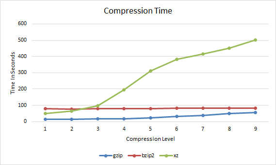
Gzip vs Bzip2 vs XZ Compression Time
So far we can see that gzip takes slightly longer to complete as the compression level increases, bzip2 does not change very much, while xz increases quite significantly after a compression level of 3.
Compression RatioNow that we have an idea of how long the compression took we can compare this with how well the file compressed. The compression ratio represents the percentage that the file has been reduced to. For example if a 100mb file has been compressed with a compression ratio of 25% it would mean that the compressed version of the file is 25mb.
gzip bzip2 xz 1 26.45 19.8 18.08 2 25.2 18.49 17.21 3 24.32 17.87 16.79 4 22.54 17.47 15.9 5 21.62 17.22 14.69 6 21.25 17.01 14.39 7 21.14 16.87 14.19 8 21.07 16.73 14.02 9 21.06 16.63 13.89 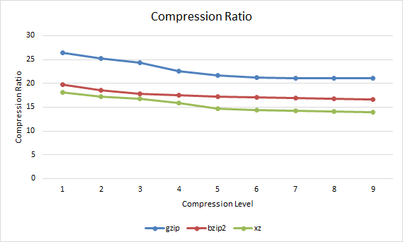
Gzip vs Bzip2 vs XZ Compression Ratio
The overall trend here is that with a higher compression level applied, the lower the compression ratio indicating that the overall file size is smaller. In this case xz is always providing the best compression ratio, closely followed by bzip2 with gzip coming in last, however as shown in the compression time graph xz takes a lot longer to get these results after compression level 3.
Compression SpeedThe compression speed in MB per second can also be observed.
gzip bzip2 xz 1 43.95 7.37 11.98 2 41.47 7.49 8.9 3 35.54 7.42 5.97 4 32.63 7.33 2.96 5 25.56 7.22 1.87 6 18.8 7.12 1.52 7 15.47 7.07 1.39 8 11.95 7.12 1.29 9 10.69 7.01 1.16 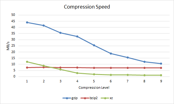
Gzip vs Bzip2 vs XZ Compression Speed Decompression Time
Next up is how long each file compressed at a particular compression level took to decompress.
gzip bzip2 xz 1 6.771 24.23 13.251 2 6.581 24.101 12.407 3 6.39 23.955 11.975 4 6.313 24.204 11.801 5 6.153 24.513 11.08 6 6.078 24.768 10.911 7 6.057 23.199 10.781 8 6.033 25.426 10.676 9 6.026 23.486 10.623 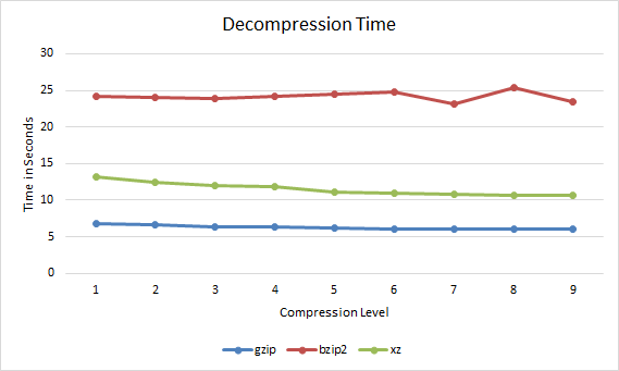
Gzip vs Bzip2 vs XZ Decompression Time
In all cases the file decompressed faster if it had been compressed with a higher compression level. Therefore if you are going to be serving out a compressed file over the Internet multiple times it may be worth compressing it with xz with a compression level of 9 as this will both reduce bandwidth over time when transferring the file, and will also be faster for everyone to decompress.
Decompression SpeedThe decompression speed in MB per second can also be observed.
1 85.77 23.97 43.83 2 88.25 24.1 46.81 3 90.9 24.24 48.5 4 91.99 24 49.21 5 94.39 23.7 52.42 6 95.55 23.45 53.23 7 95.88 25.03 53.87 8 96.26 22.84 54.4 9 96.38 24.72 54.67 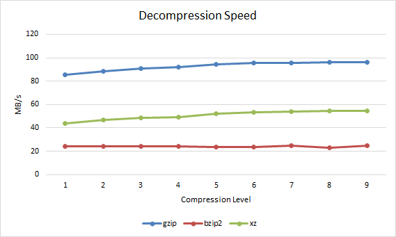
Gzip vs Bzip2 vs XZ Decompression Speed Performance Differences and Comparison
By default when the compression level is not specified, gzip uses -6, bzip2 uses -9 and xz uses -6. The reason for this is pretty clear based on the results. For gzip and xz -6 as a default compression method provides a good level of compression yet does not take too long to complete, it's a fair trade off point as higher compression levels take longer to process. Bzip2 on the other hand is best used with the default compression level of 9 as is also recommended in the manual page, the results here confirm this, the compression ratio increases but the time taken is almost the same and differs by less than a second between levels 1 to 9.
In general xz achieves the best compression level, followed by bzip2 and then gzip. In order to achieve better compression however xz usually takes the longest to complete, followed by bzip2 and then gzip.
xz takes a lot more time with its default compression level of 6 while bzip2 only takes a little longer than gzip at compression level 9 and compresses a fair amount better, while the difference between bzip2 and xz is less than the difference between bzip2 and gzip making bzip2 a good trade off for compression.
Interestingly the lowest xz compression level of 1 results in a higher compression ratio than gzip with a compression level of 9 and even completes faster. Therefore using xz with a compression level of 1 instead of gzip for a better compression ratio in a faster time.
Based on these results, bzip2 is a good middle ground for compression, gzip is only a little faster while xz may not really worth it at its higher default compression ratio of 6 as it takes much longer to complete for little extra gain.
However decompressing with bzip2 takes much longer than xz or gzip, xz is a good middle ground here while gzip is again the fastest.
ConclusionSo which should you use? It's going to come down to using the right tool for the job and the particular data set that you are working with.
If you are interactively compressing files on the fly then you may want to do this quickly with gzip -6 (default compression level) or xz -1, however if you're configuring log rotation which will run automatically over night during a low resource usage period then it may be acceptable to use more CPU resources with xz -9 to save the greatest amount of space possible. For instance kernel.org compress the Linux kernel with xz, in this case spending extra time to compress the file well once makes sense when it will be downloaded and decompressed thousands of times resulting in bandwidth savings yet still decent decompression speeds.
Based on the results here, if you're simply after being able to compress and decompress files as fast as possible with little regard to the compression ratio, then gzip is the tool for you. If you want a better compression ratio to save more disk space and are willing to spend extra processing time to get it then xz will be best to use. Although xz takes the longest to compress at higher compression levels, it has a fairly good decompression speed and compresses quite fast at lower levels. Bzip2 provides a good trade off between compression ratio and processing speed however it takes the longest to decompress so it may be a good option if the content that is being compressed will be infrequently decompressed.
In the end the best option will come down to what you're after between processing time and compression ratio. With disk space continually becoming cheaper and available in larger sizes you may be fine with saving some CPU resources and processing time to store slightly larger files. Regardless of the tool that you use, compression is a great resource for saving storage space.
May 04, 2018 | en.wikipedia.org
Lempel–Ziv–Markov chain algorithm From Wikipedia, the free encyclopedia Jump to: navigation , search "LZMA" redirects here. For the airport with the ICAO code "LZMA", see Martin Airport (Slovakia) .

hide This article has multiple issues. Please help improve it or discuss these issues on the talk page . ( Learn how and when to remove these template messages )

This article's lead section does not adequately summarize key points of its contents . Please consider expanding the lead to provide an accessible overview of all important aspects of the article. Please discuss this issue on the article's talk page . (July 2014) ( Learn how and when to remove this template message )

This article is written like a manual or guidebook . Please help rewrite this article from a descriptive, neutral point of view , and remove advice or instruction. (July 2014) ( Learn how and when to remove this template message ) The Lempel–Ziv–Markov chain algorithm ( LZMA ) is an algorithm used to perform lossless data compression . It has been under development either since 1996 or 1998 [1] and was first used in the 7z format of the 7-Zip archiver. This algorithm uses a dictionary compression scheme somewhat similar to the LZ77 algorithm published by Abraham Lempel and Jacob Ziv in 1977 and features a high compression ratio (generally higher than bzip2 ) [2] [3] and a variable compression-dictionary size (up to 4 GB ), [4] while still maintaining decompression speed similar to other commonly used compression algorithms. [5]
LZMA2 is a simple container format that can include both uncompressed data and LZMA data, possibly with multiple different LZMA encoding parameters. LZMA2 supports arbitrarily scalable multithreaded compression and decompression and efficient compression of data which is partially incompressible.
Contents [ hide ]Overview [ edit ]
- 1 Overview
- 2 Compressed format overview
- 3 Decompression algorithm details
- 4 Compression algorithm details
- 5 7-Zip reference implementation
- 6 Other implementations
- 7 LZHAM
- 8 References
- 9 External links

This section needs additional citations for verification . Please help improve this article by adding citations to reliable sources . Unsourced material may be challenged and removed. (July 2010) ( Learn how and when to remove this template message ) LZMA uses a dictionary compression algorithm (a variant of LZ77 with huge dictionary sizes and special support for repeatedly used match distances), whose output is then encoded with a range encoder , using a complex model to make a probability prediction of each bit. The dictionary compressor finds matches using sophisticated dictionary data structures, and produces a stream of literal symbols and phrase references, which is encoded one bit at a time by the range encoder: many encodings are possible, and a dynamic programming algorithm is used to select an optimal one under certain approximations.
Prior to LZMA, most encoder models were purely byte-based (i.e. they coded each bit using only a cascade of contexts to represent the dependencies on previous bits from the same byte). The main innovation of LZMA is that instead of a generic byte-based model, LZMA's model uses contexts specific to the bitfields in each representation of a literal or phrase: this is nearly as simple as a generic byte-based model, but gives much better compression because it avoids mixing unrelated bits together in the same context. Furthermore, compared to classic dictionary compression (such as the one used in zip and gzip formats), the dictionary sizes can be and usually are much larger, taking advantage of the large amount of memory available on modern systems.
Compressed format overview [ edit ]
This section needs additional citations for verification . Please help improve this article by adding citations to reliable sources . Unsourced material may be challenged and removed. (July 2010) ( Learn how and when to remove this template message ) In LZMA compression, the compressed stream is a stream of bits, encoded using an adaptive binary range coder. The stream is divided into packets, each packet describing either a single byte, or an LZ77 sequence with its length and distance implicitly or explicitly encoded. Each part of each packet is modeled with independent contexts, so the probability predictions for each bit are correlated with the values of that bit (and related bits from the same field) in previous packets of the same type.
There are 7 types of packets: [ citation needed ]
packed code (bit sequence) packet name packet description 0 + byteCode LIT A single byte encoded using an adaptive binary range coder. 1+0 + len + dist MATCH A typical LZ77 sequence describing sequence length and distance. 1+1+0+0 SHORTREP A one-byte LZ77 sequence. Distance is equal to the last used LZ77 distance. 1+1+0+1 + len LONGREP[0] An LZ77 sequence. Distance is equal to the last used LZ77 distance. 1+1+1+0 + len LONGREP[1] An LZ77 sequence. Distance is equal to the second last used LZ77 distance. 1+1+1+1+0 + len LONGREP[2] An LZ77 sequence. Distance is equal to the third last used LZ77 distance. 1+1+1+1+1 + len LONGREP[3] An LZ77 sequence. Distance is equal to the fourth last used LZ77 distance. LONGREP[*] refers to LONGREP[0-3] packets, *REP refers to both LONGREP and SHORTREP, and *MATCH refers to both MATCH and *REP.
LONGREP[n] packets remove the distance used from the list of the most recent distances and reinsert it at the front, to avoid useless repeated entry, while MATCH just adds the distance to the front even if already present in the list and SHORTREP and LONGREP[0] don't alter the list.
The length is encoded as follows:
Length code (bit sequence) Description 0+ 3 bits The length encoded using 3 bits, gives the lengths range from 2 to 9. 1+0+ 3 bits The length encoded using 3 bits, gives the lengths range from 10 to 17. 1+1+ 8 bits The length encoded using 8 bits, gives the lengths range from 18 to 273. As in LZ77, the length is not limited by the distance, because copying from the dictionary is defined as if the copy was performed byte by byte, keeping the distance constant.
Distances are logically 32-bit and distance 0 points to the most recently added byte in the dictionary.
The distance encoding starts with a 6-bit "distance slot", which determines how many further bits are needed. Distances are decoded as a binary concatenation of, from most to least significant, two bits depending on the distance slot, some bits encoded with fixed 0.5 probability, and some context encoded bits, according to the following table (distance slots 0−3 directly encode distances 0−3).
Decompression algorithm details [ edit ]
6-bit distance slot Highest 2 bits Fixed 0.5 probability bits Context encoded bits 0 00 0 0 1 01 0 0 2 10 0 0 3 11 0 0 4 10 0 1 5 11 0 1 6 10 0 2 7 11 0 2 8 10 0 3 9 11 0 3 10 10 0 4 11 11 0 4 12 10 0 5 13 11 0 5 14–62 (even) 10 ((slot / 2) − 5) 4 15–63 (odd) 11 (((slot − 1) / 2) − 5) 4
This section possibly contains original research . Please improve it by verifying the claims made and adding inline citations . Statements consisting only of original research should be removed. (April 2012) ( Learn how and when to remove this template message ) No complete natural language specification of the compressed format seems to exist, other than the one attempted in the following text.
The description below is based on the compact XZ Embedded decoder by Lasse Collin included in the Linux kernel source [6] from which the LZMA and LZMA2 algorithm details can be relatively easily deduced: thus, while citing source code as reference isn't ideal, any programmer should be able to check the claims below with a few hours of work.
Range coding of bits [ edit ]LZMA data is at the lowest level decoded one bit at a time by the range decoder, at the direction of the LZMA decoder.
Context-based range decoding is invoked by the LZMA algorithm passing it a reference to the "context", which consists of the unsigned 11-bit variable prob (typically implemented using a 16-bit data type) representing the predicted probability of the bit being 0, which is read and updated by the range decoder (and should be initialized to 2^10, representing 0.5 probability).
Fixed probability range decoding instead assumes a 0.5 probability, but operates slightly differently from context-based range decoding.
The range decoder state consists of two unsigned 32-bit variables, range (representing the range size), and code (representing the encoded point within the range).
Initialization of the range decoder consists of setting range to 2 32 − 1, and code to the 32-bit value starting at the second byte in the stream interpreted as big-endian; the first byte in the stream is completely ignored.
Normalization proceeds in this way:
- Shift both range and code left by 8 bits
- Read a byte from the compressed stream
- Set the least significant 8 bits of code to the byte value read
Context-based range decoding of a bit using the prob probability variable proceeds in this way:
- If range is less than 2^24, perform normalization
- Set bound to floor( range / 2^11) * prob
- If code is less than bound :
- Set range to bound
- Set prob to prob + floor((2^11 - prob ) / 2^5)
- Return bit 0
- Otherwise (if code is greater than or equal to the bound ):
- Set range to range - bound
- Set code to code - bound
- Set prob to prob - floor( prob / 2^5)
- Return bit 1
Fixed-probability range decoding of a bit proceeds in this way:
- If range is less than 2^24, perform normalization
- Set range to floor( range / 2)
- If code is less than range :
- Return bit 0
- Otherwise (if code is greater or equal than range ):
- Set code to code - range
- Return bit 1
The Linux kernel implementation of fixed-probability decoding in rc_direct, for performance reasons, doesn't include a conditional branch, but instead subtracts range from code unconditionally, and uses the resulting sign bit to both decide the bit to return, and to generate a mask that is combined with code and added to range .
Note that:
Range coding of integers [ edit ]
- The division by 2^11 when computing bound and floor operation is done before the multiplication, not after (apparently to avoid requiring fast hardware support for 32-bit multiplication with a 64-bit result)
- Fixed probability decoding is not strictly equivalent to context-based range decoding with any prob value, due to the fact that context-based range decoding discards the lower 11 bits of range before multiplying by prob as just described, while fixed probability decoding only discards the last bit
The range decoder also provides the bit-tree, reverse bit-tree and fixed probability integer decoding facilities, which are used to decode integers, and generalize the single-bit decoding described above. To decode unsigned integers less than limit , an array of ( limit − 1) 11-bit probability variables is provided, which are conceptually arranged as the internal nodes of a complete binary tree with limit leaves.
Non-reverse bit-tree decoding works by keeping a pointer to the tree of variables, which starts at the root. As long as the pointer doesn't point to a leaf, a bit is decoded using the variable indicated by the pointer, and the pointer is moved to either the left or right children depending on whether the bit is 0 or 1; when the pointer points to a leaf, the number associated with the leaf is returned.
Non-reverse bit-tree decoding thus happens from most significant to least significant bit, stopping when only one value in the valid range is possible (this conceptually allows to have range sizes that are not powers of two, even though LZMA doesn't make use of this).
Reverse bit-tree decoding instead decodes from least significant bit to most significant bits, and thus only supports ranges that are powers of two, and always decodes the same number of bits. It is equivalent to performing non-reverse bittree decoding with a power of two limit , and reversing the last log2( limit ) bits of the result.
Note that in the rc_bittree function in the Linux kernel, integers are actually returned in the [ limit , 2 * limit ) range (with limit added to the conceptual value), and the variable at index 0 in the array is unused, while the one at index 1 is the root, and the left and right children indices are computed as 2 i and 2 i + 1. The rc_bittree_reverse function instead adds integers in the [0, limit ) range to a caller-provided variable, where limit is implicitly represented by its logarithm, and has its own independent implementation for efficiency reasons.
Fixed probability integer decoding simply performs fixed probability bit decoding repeatedly, reading bits from the most to the least significant.
LZMA configuration [ edit ]The LZMA decoder is configured by an lclppb "properties" byte and a dictionary size.
The value of the lclppb byte is lc + lp * 9 + pb * 9 * 5, where:
- lc is the number of high bits of the previous byte to use as a context for literal encoding (the default value used by the LZMA SDK is 3)
- lp is the number of low bits of the dictionary position to include in literal_pos_state (the default value used by the LZMA SDK is 0)
- pb is the number of low bits of the dictionary position to include in pos_state (the default value used by the LZMA SDK is 2)
In non-LZMA2 streams, lc must not be greater than 8, and lp and pb must not be greater than 4. In LZMA2 streams, ( lc + lp ) and pb must not be greater than 4.
In the 7-zip LZMA file format, configuration is performed by a header containing the "properties" byte followed by the 32-bit little-endian dictionary size in bytes. In LZMA2, the properties byte can optionally be changed at the start of LZMA2 LZMA packets, while the dictionary size is specified in the LZMA2 header as later described.
LZMA coding contexts [ edit ]The LZMA packet format has already been described, and this section specifies how LZMA statistically models the LZ-encoded streams, or in other words which probability variables are passed to the range decoder to decode each bit.
Those probability variables are implemented as multi-dimensional arrays; before introducing them, a few values that are used as indices in these multidimensional arrays are defined.
The state value is conceptually based on which of the patterns in the following table match the latest 2-4 packet types seen, and is implemented as a state machine state updated according to the transition table listed in the table every time a packet is output.
The initial state is 0, and thus packets before the beginning are assumed to be LIT packets.
state previous packets next state when next packet is 4th previous 3rd previous 2nd previous previous LIT MATCH LONGREP[*] SHORTREP 0 LIT LIT LIT 0 7 8 9 1 MATCH LIT LIT 0 7 8 9 2 LONGREP[*] LIT LIT 0 7 8 9 *MATCH SHORTREP 3 LIT SHORTREP LIT LIT 0 7 8 9 4 MATCH LIT 1 7 8 9 5 LONGREP[*] LIT 2 7 8 9 *MATCH SHORTREP 6 LIT SHORTREP LIT 3 7 8 9 7 LIT MATCH 4 10 11 11 8 LIT LONGREP[*] 5 10 11 11 9 LIT SHORTREP 6 10 11 11 10 *MATCH MATCH 4 10 11 11 11 *MATCH *REP 5 10 11 11 The pos_state and literal_pos_state values consist of respectively the pb and lp (up to 4, from the LZMA header or LZMA2 properties packet) least significant bits of the dictionary position (the number of bytes coded since the last dictionary reset modulo the dictionary size). Note that the dictionary size is normally the multiple of a large power of 2, so these values are equivalently described as the least significant bits of the number of uncompressed bytes seen since the last dictionary reset.
The prev_byte_lc_msbs value is set to the lc (up to 4, from the LZMA header or LZMA2 properties packet) most significant bits of the previous uncompressed byte.
The is_REP value denotes whether a packet that includes a length is a LONGREP rather than a MATCH.
The match_byte value is the byte that would have been decoded if a SHORTREP packet had been used (in other words, the byte found at the dictionary at the last used distance); it is only used just after a *MATCH packet.
literal_bit_mode is an array of 8 values in the 0-2 range, one for each bit position in a byte, which are 1 or 2 if the previous packet was a *MATCH and it is either the most significant bit position or all the more significant bits in the literal to encode/decode are equal to the bits in the corresponding positions in match_byte , while otherwise it is 0; the choice between the 1 or 2 values depends on the value of the bit at the same position in match_byte .
The literal/Literal set of variables can be seen as a "pseudo-bit-tree" similar to a bit-tree but with 3 variables instead of 1 in every node, chosen depending on the literal_bit_mode value at the bit position of the next bit to decode after the bit-tree context denoted by the node.
The claim, found in some sources, that literals after a *MATCH are coded as the XOR of the byte value with match_byte is incorrect; they are instead coded simply as their byte value, but using the pseudo-bit-tree just described and the additional context listed in the table below.
The probability variable groups used in LZMA are those:
LZMA2 format [ edit ]
XZ name LZMA SDK name parameterized by used when coding mode if bit 0 then if bit 1 then is_match IsMatch state , pos_state packet start bit LIT *MATCH is_rep IsRep state after bit sequence 1 bit MATCH *REP is_rep0 IsRepG0 state after bit sequence 11 bit SHORTREP/ LONGREP[0]
LONGREP[1-3] is_rep0_long IsRep0Long state , pos_state after bit sequence 110 bit SHORTREP LONGREP[0] is_rep1 IsRepG1 state after bit sequence 111 bit LONGREP[1] LONGREP[2/3] is_rep2 IsRepG2 state after bit sequence 1111 bit LONGREP[2] LONGREP[3] literal Literal prev_byte_lc_msbs , literal_pos_state , literal_bit_mode [bit position], bit-tree context after bit sequence 0 256 values pseudo-bit-tree literal byte value dist_slot PosSlot min( match_length , 5), bit-tree context distance: start 64 values bit-tree distance slot dist_special SpecPos distance_slot , reverse bit-tree context distance: 4-13 distance slots (( distance_slot >> 1) − 1)-bit reverse bit-tree low bits of distance dist_align Align reverse bit-tree context distance: 14+ distance slots, after fixed probability bits 4-bit reverse bit-tree low bits of distance len_dec.choice LenChoice is_REP match length: start bit 2-9 length 10+ length len_dec.choice2 LenChoice2 is_REP match length: after bit sequence 1 bit 10-17 length 18+ length len_dec.low LenLow is_REP , pos_state , bit-tree context match length: after bit sequence 0 8 values bit-tree low bits of length len_dec.mid LenMid is_REP , pos_state , bit-tree context match length: after bit sequence 10 8 values bit-tree middle bits of length len_dec.high LenHigh is_REP , bit-tree context match length: after bit sequence 11 256 values bit-tree high bits of length The LZMA2 container supports multiple runs of compressed LZMA data and uncompressed data. Each LZMA compressed run can have a different LZMA configuration and dictionary. This improves the compression of partially or completely incompressible files and allows multithreaded compression and multithreaded decompression by breaking the file into runs that can be compressed or decompressed independently in parallel.
The LZMA2 header consists of a byte indicating the dictionary size:
- 40 indicates a 4 GB − 1 dictionary size
- Even values less than 40 indicate a 2 v /2 + 12 bytes dictionary size
- Odd values less than 40 indicate a 3×2 ( v − 1)/2 + 11 bytes dictionary size
- Values higher than 40 are invalid
LZMA2 data consists of packets starting with a control byte, with the following values:
- 0 denotes the end of the file
- 1 denotes a dictionary reset followed by an uncompressed chunk
- 2 denotes an uncompressed chunk without a dictionary reset
- 3-0x7f are invalid values
- 0x80-0xff denotes an LZMA chunk, where the lowest 5 bits are used as bit 16-20 of the uncompressed size minus one, and bit 5-6 indicates what should be reset
Bits 5-6 for LZMA chunks can be:
- 0: nothing reset
- 1: state reset
- 2: state reset, properties reset using properties byte
- 3: state reset, properties reset using properties byte, dictionary reset
LZMA state resets cause a reset of all LZMA state except the dictionary, and specifically:
- The range coder
- The state value
- The last distances for repeated matches
- All LZMA probabilities
Uncompressed chunks consist of:
- A 16-bit big-endian value encoding the data size minus one
- The data to be copied verbatim into the dictionary and the output
LZMA chunks consist of:
xz and 7z formats [ edit ]
- A 16-bit big-endian value encoding the low 16-bits of the uncompressed size minus one
- A 16-bit big-endian value encoding the compressed size minus one
- A properties/lclppb byte if bit 6 in the control byte is set
- The LZMA compressed data, starting with the 5 bytes (of which the first is ignored) used to initialize the range coder (which are included in the compressed size)
The . xz format, which can contain LZMA2 data, is documented at tukaani.org , [7] while the .7z file format, which can contain either LZMA or LZMA2 data, is documented in the 7zformat.txt file contained in the LZMA SDK. [8]
Compression algorithm details [ edit ]Similar to the decompression format situation, no complete natural language specification of the encoding techniques in 7-zip or xz seems to exist, other than the one attempted in the following text.
The description below is based on the XZ for Java encoder by Lasse Collin, [9] which appears to be the most readable among several rewrites of the original 7-zip using the same algorithms: again, while citing source code as reference isn't ideal, any programmer should be able to check the claims below with a few hours of work.
Range encoder [ edit ]The range encoder cannot make any interesting choices, and can be readily constructed based on the decoder description.
Initialization and termination are not fully determined; the xz encoder outputs 0 as the first byte which is ignored by the decompressor, and encodes the lower bound of the range (which matters for the final bytes).
The xz encoder uses an unsigned 33-bit variable called low (typically implemented as a 64-bit integer, initialized to 0), an unsigned 32-bit variable called range (initialized to 2 32 − 1), an unsigned 8-bit variable called cache (initialized to 0), and an unsigned variable called cache_size which needs to be large enough to store the uncompressed size (initialized to 1, typically implemented as a 64-bit integer).
The cache / cache_size variables are used to properly handle carries, and represent a number defined by a big-endian sequence starting with the cache value, and followed by cache_size 0xff bytes, which has been shifted out of the low register, but hasn't been written yet, because it could be incremented by one due to a carry.
Note that the first byte output will always be 0 due to the fact that cache and low are initialized to 0, and the encoder implementation; the xz decoder ignores this byte.
Normalization proceeds in this way:
- If low is less than (2^32 - 2^24):
- Output the byte stored in cache to the compressed stream
- Output cache_size - 1 bytes with 0xff value
- Set cache to bits 24-31 of low
- Set cache_size to 0
- If low is greater or equal than 2^32:
- Output the byte stored in cache plus one to the compressed stream
- Output cache_size - 1 bytes with 0 value
- Set cache to bits 24-31 of low
- Set cache_size to 0
- Increment cache_size
- Set low to the lowest 24 bits of low shifted left by 8 bits
- Set range to range shifted left by 8 bits
Context-based range encoding of a bit using the prob probability variable proceeds in this way:
- If range is less than 2^24, perform normalization
- Set bound to floor( range / 2^11) * prob
- If encoding a 0 bit:
- Set range to bound
- Set prob to prob + floor((2^11 - prob ) / 2^5)
- Otherwise (if encoding a 1 bit):
- Set range to range - bound
- Set low to low + bound
- Set prob to prob - floor( prob / 2^5)
Fixed-probability range encoding of a bit proceeds in this way:
- If range is less than 2^24, perform normalization
- Set range to floor( range / 2)
- If encoding a 1 bit:
- Set low to low + range
Termination proceeds this way:
- Perform normalization 5 times
Bit-tree encoding is performed like decoding, except that bit values are taken from the input integer to be encoded rather than from the result of the bit decoding functions.
For algorithms that try to compute the encoding with the shortest post-range-encoding size, the encoder also needs to provide an estimate of that.
Dictionary search data structures [ edit ]The encoder needs to be able to quickly locate matches in the dictionary. Since LZMA uses very large dictionaries (potentially on the order of gigabytes) to improve compression, simply scanning the whole dictionary would result in an encoder too slow to be practically usable, so sophisticated data structures are needed to support fast match searches.
Hash chains [ edit ]The simplest approach, called "hash chains", is parameterized by a constant N which can be either 2, 3 or 4, which is typically chosen so that 2^(8× N ) is greater than or equal to the dictionary size.
It consists of creating, for each k less than or equal to N , a hash table indexed by tuples of k bytes, where each of the buckets contains the last position where the first k bytes hashed to the hash value associated with that hash table bucket.
Chaining is achieved by an additional array which stores, for every dictionary position, the last seen previous position whose first N bytes hash to the same value of the first N bytes of the position in question.
To find matches of length N or higher, a search is started using the N -sized hash table, and continued using the hash chain array; the search stop after a pre-defined number of hash chain nodes has been traversed, or when the hash chains "wraps around", indicating that the portion of the input that has been overwritten in the dictionary has been reached.
Matches of size less than N are instead found by simply looking at the corresponding hash table, which either contains the latest such match, if any, or a string that hashes to the same value; in the latter case, the encoder won't be able to find the match. This issue is mitigated by the fact that for distant short matches using multiple literals might require less bits, and having hash conflicts in nearby strings is relatively unlikely; using larger hash tables or even direct lookup tables can reduce the problem at the cost of higher cache miss rate and thus lower performance.
Note that all matches need to be validated to check that the actual bytes match currently at that specific dictionary position match, since the hashing mechanism only guarantees that at some past time there were characters hashing to the hash table bucket index (some implementations may not even guarantee that, because they don't initialize the data structures).
LZMA uses Markov chains , as implied by "M" in its name.
Binary trees [ edit ]The binary tree approach follows the hash chain approach, except that it logically uses a binary tree instead of a linked list for chaining.
The binary tree is maintained so that it is always both a search tree relative to the suffix lexicographic ordering, and a max-heap for the dictionary position [10] (in other words, the root is always the most recent string, and a child cannot have been added more recently than its parent): assuming all strings are lexicographically ordered, these conditions clearly uniquely determine the binary tree (this is trivially provable by induction on the size of the tree).
Since the string to search for and the string to insert are the same, it is possible to perform both dictionary search and insertion (which requires to rotate the tree) in a single tree traversal.
Patricia tries [ edit ]Some old LZMA encoders also supported a data structure based on Patricia tries , but such support has since been dropped since it was deemed inferior to the other options. [10]
LZMA encoder [ edit ]LZMA encoders can freely decide which match to output, or whether to ignore the presence of matches and output literals anyway.
The ability to recall the 4 most recently used distances means that, in principle, using a match with a distance that will be needed again later may be globally optimal even if it is not locally optimal, and as a result of this, optimal LZMA compression probably requires knowledge of the whole input and might require algorithms too slow to be usable in practice.
Due to this, practical implementations tend to employ non-global heuristics.
The xz encoders use a value called nice_len (the default is 64): when any match of length at least nice_len is found, the encoder stops the search and outputs it, with the maximum matching length.
Fast encoder [ edit ]The XZ fast encoder [11] (derived from the 7-zip fast encoder) is the shortest LZMA encoder in the xz source tree.
It works like this:
- Perform combined search and insertion in the dictionary data structure
- If any repeated distance matches with length at least nice_len :
- Output the most frequently used such distance with a REP packet
- If a match was found of length at least nice_len :
- Output it with a MATCH packet
- Set the main match to the longest match
- Look at the nearest match of every length in decreasing length order, and until no replacement can be made:
- Replace the main match with a match which is one character shorter, but whose distance is less than 1/128 the current main match distance
- Set the main match length to 1 if the current main match is of length 2 and distance at least 128
- If a repeated match was found, and it is shorter by at most 1 character than the main match:
- Output the repeated match with a REP packet
- If a repeated match was found, and it is shorter by at most 2 characters than the main match, and the main match distance is at least 512:
- Output the repeated match with a REP packet
- If a repeated match was found, and it is shorter by at most 3 characters than the main match, and the main match distance is at least 32768:
- Output the repeated match with a REP packet
- If the main match size is less than 2 (or there isn't any match):
- Output a LIT packet
- Perform a dictionary search for the next byte
- If the next byte is shorter by at most 1 character than the main match, with distance less than 1/128 times the main match distance, and if the main match length is at least 3:
- Output a LIT packet
- If the next byte has a match at least as long as the main match, and with less distance than the main match:
- Output a LIT packet
- If the next byte has a match at least one character longer than the main match, and such that 1/128 of its distance is less or equal than the main match distance:
- Output a LIT packet
- If the next byte has a match more than one character longer than the main match:
- Output a LIT packet
- If any repeated match is shorter by at most 1 character than the main match:
- Output the most frequently used such distance with a REP packet
- Output the main match with a MATCH packet
Normal encoder [ edit ]The XZ normal encoder [12] (derived from the 7-zip normal encoder) is the other LZMA encoder in the xz source tree, which adopts a more sophisticated approach that tries to minimize the post-range-encoding size of the generated packets.
Specifically, it encodes portions of the input using the result of a dynamic programming algorithm, where the subproblems are finding the approximately optimal encoding (the one with minimal post-range-encoding size) of the substring of length L starting at the byte being compressed.
The size of the portion of the input processed in the dynamic programming algorithm is determined to be the maximum between the longest dictionary match and the longest repeated match found at the start position (which is capped by the maximum LZMA match length, 273); furthermore, if a match longer than nice_len is found at any point in the range just defined, the dynamic programming algorithm stops, the solution for the subproblem up to that point is output, the nice_len -sized match is output, and a new dynamic programming problem instance is started at the byte after the match is output.
Subproblem candidate solutions are incrementally updated with candidate encodings, constructed taking the solution for a shorter substring of length L', extended with all possible "tails", or sets of 1-3 packets with certain constraints that encode the input at the L' position. Once the final solution of a subproblem is found, the LZMA state and least used distances for it are computed, and are then used to appropriately compute post-range-encoding sizes of its extensions.
At the end of the dynamic programming optimization, the whole optimal encoding of the longest substring considered is output, and encoding continues at the first uncompressed byte not already encoded, after updating the LZMA state and least used distances.
Each subproblem is extended by a packet sequence which we call "tail", which must match one of the following patterns:
1st packet 2nd packet 3rd packet any LIT LONGREP[0] *MATCH LIT LONGREP[0] The reason for not only extending with single packets is that subproblems only have the substring length as the parameter for performance and algorithmic complexity reasons, while an optimal dynamic programming approach would also require to have the last used distances and LZMA state as parameter; thus, extending with multiple packets allows to better approximate the optimal solution, and specifically to make better use of LONGREP[0] packets.
The following data is stored for each subproblem (of course, the values stored are for the candidate solution with minimum price ), where by "tail" we refer to the packets extending the solution of the smaller subproblem, which are described directly in the following structure:
XZ for Java member name description price quantity to be minimized: number of post-range-encoding bits needed to encode the string optPrev uncompressed size of the substring encoded by all packets except the last one backPrev -1 if the last packet is LIT, 0-3 if it is a repetition using the last used distance number 0-3, 4 + distance if it is a MATCH (this is always 0 if prev1IsLiteral is true, since the last packet can only be a LONGREP[0] in that case) prev1IsLiteral true if the "tail" contains more than one packet (in which case the one before the last is a LIT) hasPrev2 true if the "tail" contains 3 packets (only valid if prev1IsLiteral is true) optPrev2 uncompressed size of the substring encoded by all packets except the "tail" (only valid if prev1IsLiteral and hasPrev2 are true) backPrev2 -1 if the first packet in the "tail" is LIT, 0-3 if it is a repetition using the last used distance number 0-3, 4 + distance if it is a MATCH (only valid if prev1IsLiteral and hasPrev2 are true) reps[4] the values of the 4 last used distances after the packets in the solution (computed only after the best subproblem solution has been determined) state the LZMA state value after the packets in the solution (computed only after the best subproblem solution has been determined) Note that in the XZ for Java implementation, the optPrev and backPrev members are reused to store a forward single-linked list of packets as part of outputting the final solution.
LZMA2 encoder [ edit ]The XZ LZMA2 encoder processes the input in chunks (of up to 2 MB uncompressed size or 64 KB compressed size, whichever is lower), handing each chunk to the LZMA encoder, and then deciding whether to output an LZMA2 LZMA chunk including the encoded data, or to output an LZMA2 uncompressed chunk, depending on which is shorter (LZMA, like any other compressor, will necessarily expand rather than compress some kinds of data).
The LZMA state is reset only in the first block, if the caller requests a change of properties and every time a compressed chunk is output. The LZMA properties are changed only in the first block, or if the caller requests a change of properties. The dictionary is only reset in the first block.
Upper encoding layers [ edit ]Before LZMA2 encoding, depending on the options provided, xz can apply the BCJ filter, which filters executable code to replace relative offsets with absolute ones that are more repetitive, or the delta filter, which replaces each byte with the difference between it and the byte N bytes before it.
Parallel encoding is performed by dividing the file in chunks which are distributed to threads, and ultimately each encoded (using, for instance, xz block encoding) separately, resulting in a dictionary reset between chunks in the output file.
7-Zip reference implementation [ edit ]The LZMA implementation extracted from 7-Zip is available as LZMA SDK. It was originally dual-licensed under both the GNU LGPL and Common Public License , [13] with an additional special exception for linked binaries, but was placed by Igor Pavlov in the public domain on December 2, 2008, with the release of version 4.62. [8]
LZMA2 compression, which is an improved version of LZMA, [14] is now the default compression method for the .7z format, starting with version 9.30 on October 26th, 2012. [15]
The reference open source LZMA compression library is written in C++ and has the following properties:
- Compression speed: approximately 1 MB/s on a 2 GHz CPU .
- Decompression speed: 10–20 MB/s on a 2 GHz CPU.
- Support for multithreading .
In addition to the original C++ , the LZMA SDK contains reference implementations of LZMA compression and decompression ported to ANSI C , C# , and Java . [8] There are also third-party Python bindings for the C++ library, as well as ports of LZMA to Pascal , Go and Ada . [16] [17] [18] [19]
The 7-Zip implementation uses several variants of hash chains , binary trees and Patricia tries as the basis for its dictionary search algorithm.
Decompression-only code for LZMA generally compiles to around 5 KB, and the amount of RAM required during decompression is principally determined by the size of the sliding window used during compression. Small code size and relatively low memory overhead, particularly with smaller dictionary lengths, and free source code make the LZMA decompression algorithm well-suited to embedded applications.
Other implementations [ edit ]In addition to the 7-Zip reference implementation, the following support the LZMA format.
LZHAM [ edit ]
- xz : a streaming implementation that contains a gzip -like command line tool, supporting both LZMA and LZMA2 in its xz file format. It made its way into several software of the Unix-like world with its high performance (compared to bzip2 ) and small size (compared to gzip ). [2] The Linux kernel , dpkg and RPM systems contains xz code, and many software distributors like kernel.org , Debian [20] and Fedora now use xz for compressing their releases.
- lzip : another LZMA implementation mostly for Unix-like systems to be directly competing with xz . [21] It mainly features a simpler file format and therefore easier error recovery.
- ZIPX : an extension to the ZIP compressions format that was created by WinZip starting with version 12.1. It also can use various other compression methods such as BZip and PPMd . [22]
- DotNetCompression : a streaming implementation of LZMA in managed C#.
LZHAM (LZ, Huffman, Arithmetic, Markov), is an LZMA-like implementation that trades compression throughput for very high ratios and higher decompression throughput. [23]
References [ edit ]External links [ edit ]
- Jump up ^ Igor Pavlov has asserted multiple times on SourceForge that the algorithm is his own creation. (2004-02-19). "LZMA spec?" . Archived from the original on 2009-08-25 . Retrieved 2013-06-16 .
- ^ Jump up to: a b Lasse Collin (2005-05-31). "A Quick Benchmark: Gzip vs. Bzip2 vs. LZMA" . Retrieved 2015-10-21 . - LZMA Unix Port was finally replaced by xz which features better and faster compression; from here we know even LZMA Unix Port was a lot better than gzip and bzip2.
- Jump up ^ Klausmann, Tobias (2008-05-08). "Gzip, Bzip2 and Lzma compared" . Blog of an Alpha animal . Retrieved 2013-06-16 .
- Jump up ^ Igor Pavlov (2013). "7z Format" . Retrieved 2013-06-16 .
- Jump up ^ Mahoney, Matt. "Data Compression Explained" . Retrieved 2013-11-13 .
- Jump up ^ Collin, Lasse; Pavlov, Igor. "lib/xz/xz_dec_lzma2.c" . Retrieved 2013-06-16 .
- Jump up ^ "The .xz File Format" . 2009-08-27 . Retrieved 2013-06-16 .
- ^ Jump up to: a b c Igor Pavlov (2013). "LZMA SDK (Software Development Kit)" . Retrieved 2013-06-16 .
- Jump up ^ "XZ in Java" . Retrieved 2013-06-16 . [ permanent dead link ]
- ^ Jump up to: a b Solomon, David (2006-12-19). Data Compression: The Complete Reference (4 ed.). Springer Publishing . p. 245. ISBN 978-1846286025 .
- Jump up ^ Collin, Lasse; Pavlov, Igor. "LZMAEncoderFast.java" . Archived from the original on 2012-07-16 . Retrieved 2013-06-16 .
- Jump up ^ Collin, Lasse; Pavlov, Igor. "LZMAEncoderNormal.java" . Archived from the original on 2012-07-08 . Retrieved 2013-06-16 .
- Jump up ^ "Browse /LZMA SDK/4.23" . Sourceforge . Retrieved 2014-02-12 .
- Jump up ^ "Inno Setup Help" . jrsoftware.org . Retrieved 2013-06-16 .
LZMA2 is a modified version of LZMA that offers a better compression ratio for uncompressible data (random data expands about 0.005%, compared to 1.35% with original LZMA), and optionally can compress multiple parts of large files in parallel, greatly increasing compression speed but with a possible reduction in compression ratio.- Jump up ^ "HISTORY of the 7-Zip" . 2012-10-26 . Retrieved 2013-06-16 .
- Jump up ^ Bauch, Joachim (2010-04-07). "PyLZMA – Platform independent python bindings for the LZMA compression library" . Retrieved 2013-06-16 .
- Jump up ^ Birtles, Alan (2006-06-13). "Programming Help: Pascal LZMA SDK" . Retrieved 2013-06-16 .
- Jump up ^ Vieru, Andrei (2012-06-28). "compress/lzma package for Go 1" . Retrieved 2013-06-16 .
- Jump up ^ "Zip-Ada" .
- Jump up ^ Guillem Jover. "Accepted dpkg 1.17.0 (source amd64 all)" . Debian Package QA . Retrieved 2015-10-21 .
- Jump up ^ Diaz, Diaz. "Lzip Benchmarks" . LZIP (nongnu).
- Jump up ^ "What is a Zipx File?" . WinZip.com . Retrieved 2016-03-14 .
- Jump up ^ "LZHAM – Lossless Data Compression Codec" . Richard Geldreich.
LZHAM is a lossless data compression codec written in C/C++ with a compression ratio similar to LZMA but with 1.5x-8x faster decompression speed.
- Official home page
- Lzip format specification
- XZ format specification
- LZMA SDK (Software Development Kit)
- LZMA Utils = XZ Utils
- Windows Binaries for XZ Utils
- Data compression, Compressors & Archivers
[ show ] Archive formats Archiving only Compression only Archiving and compression Software packaging and distribution Document packaging and distribution Retrieved from " https://en.wikipedia.org/w/index.php?title=Lempel–Ziv–Markov_chain_algorithm&oldid=831085554 " Categories : Hidden categories:
[ show ] Data compression methods Lossless
Entropy type Dictionary type Other types Audio
Concepts Codec parts Image
Concepts Methods Video
Concepts Codec parts Theory Navigation menu Personal tools
- All articles with dead external links
- Articles with dead external links from January 2018
- Articles with permanently dead external links
- Wikipedia introduction cleanup from July 2014
- All pages needing cleanup
- Articles covered by WikiProject Wikify from July 2014
- All articles covered by WikiProject Wikify
- Wikipedia articles needing style editing from July 2014
- All articles needing style editing
- Articles with multiple maintenance issues
- Articles needing additional references from July 2010
- All articles needing additional references
- All articles with unsourced statements
- Articles with unsourced statements from June 2013
- Articles that may contain original research from April 2012
- All articles that may contain original research
Namespaces Variants Views More Navigation
- Not logged in
- Talk
- Contributions
- Create account
- Log in
Interaction Tools
- Main page
- Contents
- Featured content
- Current events
- Random article
- Donate to Wikipedia
- Wikipedia store
Print/export Languages
- What links here
- Related changes
- Upload file
- Special pages
- Permanent link
- Page information
- Wikidata item
- Cite this page
Edit links
- Български
- Català
- Čeština
- Deutsch
- Español
- Français
- 한국어
- Italiano
- Magyar
- 日本語
- Polski
- Português
- Русский
- Slovenščina
- Svenska
- 中文
- This page was last edited on 18 March 2018, at 17:37.
- Text is available under the Creative Commons Attribution-ShareAlike License ; additional terms may apply. By using this site, you agree to the Terms of Use and Privacy Policy . Wikipedia® is a registered trademark of the Wikimedia Foundation, Inc. , a non-profit organization.
- Privacy policy
- About Wikipedia
- Disclaimers
- Contact Wikipedia
- Developers
- Cookie statement
- Mobile view
- Enable previews


Mar 13, 2018 | www.linuxtoday.com
(Mar 12, 2018, 11:00) ( 0 talkbacks )
zstd is an open-source lossless data compression algorithm designed to offer fast real-time compression and decompression speeds, even faster than xz or gzip.
Dec 05, 2014 | www.youtube.comPublished on
In this video you will learn about the Knuth-Morris-Pratt (KMP) string matching algorithm, and how it can be used to find string matches super fast!
KMP Algorithm explained - YouTube
Knuth-Morris-Pratt - Pattern Matching - YouTube
Nov 15, 2017 | ics.uci.edu
ICS 161: Design and Analysis of Algorithms
Lecture notes for February 27, 1996
Knuth-Morris-Pratt string matching The problem: given a (short) pattern and a (long) text, both strings, determine whether the pattern appears somewhere in the text. Last time we saw how to do this with finite automata. This time we'll go through the Knuth - Morris - Pratt (KMP) algorithm, which can be thought of as an efficient way to build these automata. I also have some working C++ source code which might help you understand the algorithm better.First let's look at a naive solution.
suppose the text is in an array: char T[n]
and the pattern is in another array: char P[m].One simple method is just to try each possible position the pattern could appear in the text.
Naive string matching :
    for (i=0; T[i] != '\0'; i++)
    {
    for (j=0; T[i+j] != '\0' && P[j] != '\0' && T[i+j]==P[j]; j++) ;
    if (P[j] == '\0') found a match
    }
There are two nested loops; the inner one takes O(m) iterations and the outer one takes O(n) iterations so the total time is the product, O(mn). This is slow; we'd like to speed it up.In practice this works pretty well -- not usually as bad as this O(mn) worst case analysis. This is because the inner loop usually finds a mismatch quickly and move on to the next position without going through all m steps. But this method still can take O(mn) for some inputs. In one bad example, all characters in T[] are "a"s, and P[] is all "a"'s except for one "b" at the end. Then it takes m comparisons each time to discover that you don't have a match, so mn overall.
Here's a more typical example. Each row represents an iteration of the outer loop, with each character in the row representing the result of a comparison (X if the comparison was unequal). Suppose we're looking for pattern "nano" in text "banananobano".
     0  1  2  3  4  5  6  7  8  9 10 11
      T: b  a  n  a  n  a  n  o  b  a  n  o

    i=0: X
    i=1:    X
    i=2:       n  a  n  X
    i=3:          X
    i=4:             n  a  n  o
    i=5:                X
    i=6:                   n  X
    i=7:                         X
    i=8:                            X
    i=9:                               n  X
    i=10:                                 X
Some of these comparisons are wasted work! For instance, after iteration i=2, we know from the comparisons we've done that T[3]="a", so there is no point comparing it to "n" in iteration i=3. And we also know that T[4]="n", so there is no point making the same comparison in iteration i=4. Skipping outer iterations The Knuth-Morris-Pratt idea is, in this sort of situation, after you've invested a lot of work making comparisons in the inner loop of the code, you know a lot about what's in the text. Specifically, if you've found a partial match of j characters starting at position i, you know what's in positions T[i]...T[i+j-1].You can use this knowledge to save work in two ways. First, you can skip some iterations for which no match is possible. Try overlapping the partial match you've found with the new match you want to find:
    i=2: n  a  n
    i=3:    n  a  n  o
Here the two placements of the pattern conflict with each other -- we know from the i=2 iteration that T[3] and T[4] are "a" and "n", so they can't be the "n" and "a" that the i=3 iteration is looking for. We can keep skipping positions until we find one that doesn't conflict:i=2: n a n i=4: n a n oHere the two "n"'s coincide. Define the overlap of two strings x and y to be the longest word that's a suffix of x and a prefix of y. Here the overlap of "nan" and "nano" is just "n". (We don't allow the overlap to be all of x or y, so it's not "nan"). In general the value of i we want to skip to is the one corresponding to the largest overlap with the current partial match:String matching with skipped iterations :
    i=0;
    while (i<n)
    {
    for (j=0; T[i+j] != '\0' && P[j] != '\0' && T[i+j]==P[j]; j++) ;
    if (P[j] == '\0') found a match;
    i = i + max(1, j-overlap(P[0..j-1],P[0..m]));
    }
Skipping inner iterations The other optimization that can be done is to skip some iterations in the inner loop. Let's look at the same example, in which we skipped from i=2 to i=4:i=2: n a n i=4: n a n oIn this example, the "n" that overlaps has already been tested by the i=2 iteration. There's no need to test it again in the i=4 iteration. In general, if we have a nontrivial overlap with the last partial match, we can avoid testing a number of characters equal to the length of the overlap.This change produces (a version of) the KMP algorithm:
    i=0;
    o=0;
    while (i<n)
    {
    for (j=o; T[i+j] != '\0' && P[j] != '\0' && T[i+j]==P[j]; j++) ;
    if (P[j] == '\0') found a match;
    o = overlap(P[0..j-1],P[0..m]);
    i = i + max(1, j-o);
    }
The only remaining detail is how to compute the overlap function. This is a function only of j, and not of the characters in T[], so we can compute it once in a preprocessing stage before we get to this part of the algorithm. First let's see how fast this algorithm is. KMP time analysis We still have an outer loop and an inner loop, so it looks like the time might still be O(mn). But we can count it a different way to see that it's actually always less than that. The idea is that every time through the inner loop, we do one comparison T[i+j]==P[j]. We can count the total time of the algorithm by counting how many comparisons we perform.We split the comparisons into two groups: those that return true, and those that return false. If a comparison returns true, we've determined the value of T[i+j]. Then in future iterations, as long as there is a nontrivial overlap involving T[i+j], we'll skip past that overlap and not make a comparison with that position again. So each position of T[] is only involved in one true comparison, and there can be n such comparisons total. On the other hand, there is at most one false comparison per iteration of the outer loop, so there can also only be n of those. As a result we see that this part of the KMP algorithm makes at most 2n comparisons and takes time O(n).
KMP and finite automata If we look just at what happens to j during the algorithm above, it's sort of like a finite automaton. At each step j is set either to j+1 (in the inner loop, after a match) or to the overlap o (after a mismatch). At each step the value of o is just a function of j and doesn't depend on other information like the characters in T[]. So we can draw something like an automaton, with arrows connecting values of j and labeled with matches and mismatches.
The difference between this and the automata we are used to is that it has only two arrows out of each circle, instead of one per character. But we can still simulate it just like any other automaton, by placing a marker on the start state (j=0) and moving it around the arrows. Whenever we get a matching character in T[] we move on to the next character of the text. But whenever we get a mismatch we look at the same character in the next step, except for the case of a mismatch in the state j=0.
So in this example (the same as the one above) the automaton goes through the sequence of states:
    j=0
            mismatch T[0] != "n"
    j=0
            mismatch T[1] != "n"
    j=0
            match T[2] == "n"
    j=1
            match T[3] == "a"
    j=2
            match T[4] == "n"
    j=3
            mismatch T[5] != "o"
    j=1
            match T[5] == "a"
    j=2
            match T[6] == "n"
    j=3
            match T[7] == "o"
    j=4
            found match
    j=0
            mismatch T[8] != "n"
    j=0
            mismatch T[9] != "n"
    j=0
            match T[10] == "n"
    j=1
            mismatch T[11] != "a"
    j=0
            mismatch T[11] != "n"
This is essentially the same sequence of comparisons done by the KMP pseudocode above. So this automaton provides an equivalent definition of the KMP algorithm.As one student pointed out in lecture, the one transition in this automaton that may not be clear is the one from j=4 to j=0. In general, there should be a transition from j=m to some smaller value of j, which should happen on any character (there are no more matches to test before making this transition). If we want to find all occurrences of the pattern, we should be able to find an occurrence even if it overlaps another one. So for instance if the pattern were "nana", we should find both occurrences of it in the text "nanana". So the transition from j=m should go to the next longest position that can match, which is simply j=overlap(pattern,pattern). In this case overlap("nano","nano") is empty (all suffixes of "nano" use the letter "o", and no prefix does) so we go to j=0.
Alternate version of KMP The automaton above can be translated back into pseudo-code, looking a little different from the pseudo-code we saw before but performing the same comparisons.KMP, version 2 :
    j = 0;
    for (i = 0; i < n; i++)
    for (;;) {      // loop until break
        if (T[i] == P[j]) { // matches?
        j++;        // yes, move on to next state
        if (j == m) {   // maybe that was the last state
            found a match;
            j = overlap[j];
        }
        break;
        } else if (j == 0) break;   // no match in state j=0, give up
        else j = overlap[j];    // try shorter partial match
    }
The code inside each iteration of the outer loop is essentially the same as the function match from the C++ implementation I've made available. One advantage of this version of the code is that it tests characters one by one, rather than performing random access in the T[] array, so (as in the implementation) it can be made to work for stream-based input rather than having to read the whole text into memory first.The overlap[j] array stores the values of overlap(pattern[0..j-1],pattern), which we still need to show how to compute.
Since this algorithm performs the same comparisons as the other version of KMP, it takes the same amount of time, O(n). One way of proving this bound directly is to note, first, that there is one true comparison (in which T[i]==P[j]) per iteration of the outer loop, since we break out of the inner loop when this happens. So there are n of these total. Each of these comparisons results in increasing j by one. Each iteration of the inner loop in which we don't break out of the loop results in executing the statement j=overlap[j], which decreases j. Since j can only decrease as many times as it's increased, the total number of times this happens is also O(n).
Computing the overlap function Recall that we defined the overlap of two strings x and y to be the longest word that's a suffix of x and a prefix of y. The missing component of the KMP algorithm is a computation of this overlap function: we need to know overlap(P[0..j-1],P) for each value of j>0. Once we've computed these values we can store them in an array and look them up when we need them.To compute these overlap functions, we need to know for strings x and y not just the longest word that's a suffix of x and a prefix of y, but all such words. The key fact to notice here is that if w is a suffix of x and a prefix of y, and it's not the longest such word, then it's also a suffix of overlap(x,y). (This follows simply from the fact that it's a suffix of x that is shorter than overlap(x,y) itself.) So we can list all words that are suffixes of x and prefixes of y by the following loop:
    while (x != empty) {
    x = overlap(x,y);
    output x;
    }
Now let's make another definition: say that shorten(x) is the prefix of x with one fewer character. The next simple observation to make is that shorten(overlap(x,y)) is still a prefix of y, but is also a suffix of shorten(x).So we can find overlap(x,y) by adding one more character to some word that's a suffix of shorten(x) and a prefix of y. We can just find all such words using the loop above, and return the first one for which adding one more character produces a valid overlap:
Overlap computation :
    z = overlap(shorten(x),y)
    while (last char of x != y[length(z)])
    {
    if (z = empty) return overlap(x,y) = empty
    else z = overlap(z,y)
    }
    return overlap(x,y) = z
So this gives us a recursive algorithm for computing the overlap function in general. If we apply this algorithm for x=some prefix of the pattern, and y=the pattern itself, we see that all recursive calls have similar arguments. So if we store each value as we compute it, we can look it up instead of computing it again. (This simple idea of storing results instead of recomputing them is known as dynamic programming ; we discussed it somewhat in the first lecture and will see it in more detail next time .)So replacing x by P[0..j-1] and y by P[0..m-1] in the pseudocode above and replacing recursive calls by lookups of previously computed values gives us a routine for the problem we're trying to solve, of computing these particular overlap values. The following pseudocode is taken (with some names changed) from the initialization code of the C++ implementation I've made available. The value in overlap[0] is just a flag to make the rest of the loop simpler. The code inside the for loop is the part that computes each overlap value.
KMP overlap computation :
    overlap[0] = -1;
    for (int i = 0; pattern[i] != '\0'; i++) {
    overlap[i + 1] = overlap[i] + 1;
    while (overlap[i + 1] > 0 &&
           pattern[i] != pattern[overlap[i + 1] - 1])
        overlap[i + 1] = overlap[overlap[i + 1] - 1] + 1;
    }
    return overlap;
Let's finish by analyzing the time taken by this part of the KMP algorithm. The outer loop executes m times. Each iteration of the inner loop decreases the value of the formula overlap[i+1], and this formula's value only increases by one when we move from one iteration of the outer loop to the next. Since the number of decreases is at most the number of increases, the inner loop also has at most m iterations, and the total time for the algorithm is O(m).The entire KMP algorithm consists of this overlap computation followed by the main part of the algorithm in which we scan the text (using the overlap values to speed up the scan). The first part takes O(m) and the second part takes O(n) time, so the total time is O(m+n).
Published on Dec 5, 2014In this video you will learn about the Knuth-Morris-Pratt (KMP) string matching algorithm, and how it can be used to find string matches super fast!
KMP Algorithm explained - YouTube
Knuth-Morris-Pratt - Pattern Matching - YouTube
KMP Algorithm explained - YouTube
KMP Searching Algorithm - YouTube
Nov 15, 2017 | www.youtube.com
Nov 07, 2017 | www.amazon.com
sortedandlist.sortis Timsort, an adaptive algorithm that switches from insertion sort to merge sort strategies, depending on how ordered the data is. This is efficient because real-world data tends to have runs of sorted items. There is a Wikipedia article about it.Timsort was first deployed in CPython, in 2002. Since 2009, Timsort is also used to sort arrays in both standard Java and Android, a fact that became widely known when Oracle used some of the code related to Timsort as evidence of Google infringement of Sun's intellectual property. See Oracle v. Google - Day 14 Filings .
Timsort was invented by Tim Peters, a Python core developer so prolific that he is believed to be an AI, the Timbot. You can read about that conspiracy theory in Python Humor . Tim also wrote The Zen of Python:
import this.
Oct 28, 2017 | durangobill.com
//****************************************************************************
//
// Sort Algorithms
// by
// Bill Butler
//
// This program can execute various sort algorithms to test how fast they run.
//
// Sorting algorithms include:
// Bubble sort
// Insertion sort
// Median-of-three quicksort
// Multiple link list sort
// Shell sort
//
// For each of the above, the user can generate up to 10 million random
// integers to sort. (Uses a pseudo random number generator so that the list
// to sort can be exactly regenerated.)
// The program also times how long each sort takes.
//
Oct 28, 2017 | epaperpress.com
26 pages PDF. Source code in C and Visual Basic c are linked in the original paper
This is a collection of algorithms for sorting and searching. Descriptions are brief and intuitive, with just enough theory thrown in to make you nervous. I assume you know a high-level language, such as C, and that you are familiar with programming concepts including arrays and pointers.
The first section introduces basic data structures and notation. The next section presents several sorting algorithms. This is followed by a section on dictionaries, structures that allow efficient insert, search, and delete operations. The last section describes algorithms that sort data and implement dictionaries for very large files. Source code for each algorithm, in ANSI C, is included.
Most algorithms have also been coded in Visual Basic. If you are programming in Visual Basic, I recommend you read Visual Basic Collections and Hash Tables, for an explanation of hashing and node representation.
If you are interested in translating this document to another language, please send me email. Special thanks go to Pavel Dubner, whose numerous suggestions were much appreciated. The following files may be downloaded:
source code (C) (24k)
source code (Visual Basic) (27k)
Permission to reproduce portions of this document is given provided the web site listed below is referenced, and no additional restrictions apply. Source code, when part of a software project, may be used freely without reference to the author.
Thomas Niemann
Portland, Oregon epaperpress.
Contents
Contents .......................................................................................................................................... 2
Preface ............................................................................................................................................ 3
Introduction ...................................................................................................................................... 4
Arrays........................................................................................................................................... 4
Linked Lists .................................................................................................................................. 5
Timing Estimates.......................................................................................................................... 5
Summary...................................................................................................................................... 6
Sorting ............................................................................................................................................. 7
Insertion Sort................................................................................................................................ 7
Shell Sort...................................................................................................................................... 8
Quicksort ...................................................................................................................................... 9
Comparison................................................................................................................................ 11
External Sorting.......................................................................................................................... 11
Dictionaries .................................................................................................................................... 14
Hash Tables ............................................................................................................................... 14
Binary Search Trees .................................................................................................................. 18
Red-Black Trees ........................................................................................................................ 20
Skip Lists.................................................................................................................................... 23
Comparison................................................................................................................................ 24
Bibliography................................................................................................................................... 26
Announcing the first Art of Computer Programming eBooks
For many years I've resisted temptations to put out a hasty electronic version of The Art of Computer Programming, because the samples sent to me were not well made.
But now, working together with experts at Mathematical Sciences Publishers, Addison-Wesley and I have launched an electronic edition that meets the highest standards. We've put special emphasis into making the search feature work well. Thousands of useful "clickable" cross-references are also provided --- from exercises to their answers and back, from the index to the text, from the text to important tables and figures, etc.
Note: However, I have personally approved ONLY the PDF versions of these books. Beware of glitches in the ePUB and Kindle versions, etc., which cannot be faithful to my intentions because of serious deficiencies in those alternative formats. Indeed, the Kindle edition in particular is a travesty, an insult to Addison-Wesley's proud tradition of quality.
Readers of the Kindle edition should not expect the mathematics to make sense! Maybe the ePUB version is just as bad, or worse --- I don't know, and I don't really want to know. If you have been misled into purchasing any part of eTAOCP in an inferior format, please ask the publisher for a replacement.
The first fascicle can be ordered from Pearson's InformIT website, and so can Volumes 1, 2, 3, and 4A.
MMIXware
Hooray: After fifteen years of concentrated work with the help of numerous volunteers, I'm finally able to declare success by releasing Version 1.0 of the software for MMIX. This represents the most difficult set of programs I have ever undertaken to write; I regard it as a major proof-of-concept for literate programming, without which I believe the task would have been too difficult.
Version 0.0 was published in 1999 as a tutorial volume of Springer's Lecture Notes in Computer Science, Number 1750. Version 1.0 has now been published as a thoroughly revised printing, available both in hardcopy and as an eBook. I hope readers will enjoy such things as the exposition of a computer's pipeline, which is discussed via analogy to the activites in a high tech automobile repair shop. There also is a complete implementation of IEEE standard floating point arithmetic in terms of operations on 32-point integers, including original routines for floating point input and output that deliver the maximum possible accuracy. The book contains extensive indexes, designed to enhance the experience of readers who wish to exercise and improve their code-reading skills.
The MMIX Supplement

I'm pleased to announce the appearance of an excellent 200-page companion to Volumes 1, 2, and 3, written by Martin Ruckert. It is jam-packed with goodies from which an extraordinary amount can be learned. Martin has not merely transcribed my early programs for MIX and recast them in a modern idiom using MMIX; he has penetrated to their essence and rendered them anew with elegance and good taste.
His carefully checked code represents a significant contribution to the art of pedagogy as well as to the art of programming.
Wikipedia
- Introduction
- Compiler construction
- Compiler
- Interpreter
- History of compiler writing
- Lexical analysis
- Lexical analysis
- Regular expression
- Regular expression examples
- Finite-state machine
- Preprocessor
- Syntactic analysis
- Parsing
- Lookahead
- Symbol table
- Abstract syntax
- Abstract syntax tree
- Context-free grammar
- Terminal and nonterminal symbols
- Left recursion
- Backus–Naur Form
- Extended Backus–Naur Form
- TBNF
- Top-down parsing
- Recursive descent parser
- Tail recursive parser
- Parsing expression grammar
- LL parser
- LR parser
- Parsing table
- Simple LR parser
- Canonical LR parser
- GLR parser
- LALR parser
- Recursive ascent parser
- Parser combinator
- Bottom-up parsing
- Chomsky normal form
- CYK algorithm
- Simple precedence grammar
- Simple precedence parser
- Operator-precedence grammar
- Operator-precedence parser
- Shunting-yard algorithm
- Chart parser
- Earley parser
- The lexer hack
- Scannerless parsing
- Semantic analysis
- Attribute grammar
- L-attributed grammar
- LR-attributed grammar
- S-attributed grammar
- ECLR-attributed grammar
- Intermediate language
- Control flow graph
- Basic block
- Call graph
- Data-flow analysis
- Use-define chain
- Live variable analysis
- Reaching definition
- Three-address code
- Static single assignment form
- Dominator
- C3 linearization
- Intrinsic function
- Aliasing
- Alias analysis
- Array access analysis
- Pointer analysis
- Escape analysis
- Shape analysis
- Loop dependence analysis
- Program slicing
- Code optimization
- Compiler optimization
- Peephole optimization
- Copy propagation
- Constant folding
- Sparse conditional constant propagation
- Common subexpression elimination
- Partial redundancy elimination
- Global value numbering
- Strength reduction
- Bounds-checking elimination
- Inline expansion
- Return value optimization
- Dead code
- Dead code elimination
- Unreachable code
- Redundant code
- Jump threading
- Superoptimization
- Loop optimization
- Induction variable
- Loop fission
- Loop fusion
- Loop inversion
- Loop interchange
- Loop-invariant code motion
- Loop nest optimization
- Manifest expression
- Polytope model
- Loop unwinding
- Loop splitting
- Loop tiling
- Loop unswitching
- Interprocedural optimization
- Whole program optimization
- Adaptive optimization
- Lazy evaluation
- Partial evaluation
- Profile-guided optimization
- Automatic parallelization
- Loop scheduling
- Vectorization
- Superword Level Parallelism
- Code generation
- Code generation
- Name mangling
- Register allocation
- Chaitin's algorithm
- Rematerialization
- Sethi-Ullman algorithm
- Data structure alignment
- Instruction selection
- Instruction scheduling
- Software pipelining
- Trace scheduling
- Just-in-time compilation
- Bytecode
- Dynamic compilation
- Dynamic recompilation
- Object file
- Code segment
- Data segment
- .bss
- Literal pool
- Overhead code
- Link time
- Relocation
- Library
- Static build
- Architecture Neutral Distribution Format
- Development techniques
- Bootstrapping
- Compiler correctness
- Jensen's Device
- Man or boy test
- Cross compiler
- Source-to-source compiler
- Tools
- Compiler-compiler
- PQCC
- Compiler Description Language
- Comparison of regular expression engines
- Comparison of parser generators
- Lex
- Flex lexical analyser
- Quex
- Ragel
- Yacc
- Berkeley Yacc
- ANTLR
- GNU bison
- Coco/R
- GOLD
- JavaCC
- JetPAG
- Lemon Parser Generator
- LALR parser generator
- ROSE compiler framework
- SableCC
- Scannerless Boolean Parser
- Spirit Parser Framework
- S/SL programming language
- SYNTAX
- Syntax Definition Formalism
- TREE-META
- Frameworks supporting the polyhedral model
- Case studies
- GNU Compiler Collection
- Java performance
- Literature
- Compilers: Principles, Techniques, and Tools
- Principles of Compiler Design
- The Design of an Optimizing Compiler
Amazon.com/ O'Reilly
K. Jazayeri (San Jose, CA United States): Its pedestrian title gives a very wrong first-impression!, December 12, 2008
In recent years I have found most other non-textbooks on algorithms to be uninteresting mainly for two reasons. First, there are books that are re-released periodically in a new "programming language du jour" without adding real value (some moving from Pascal to C/C++ to Python, Java or C#). The second group are books that are rather unimaginative collections of elementary information, often augmenting their bulk with lengthy pages of source code (touted as "ready-to-use", but never actually usable).
I almost didn't pay any attention to this book because its title struck me as rather mundane and pedestrian .... what an uncommonly false first-impression that turned out to be!
The is a well-written book and a great practical and usable one for working software developers at any skill or experience level. It starts with a condensed set of introductory material. It then covers the gamut of common and some not-so-common algorithms grouped by problems/tasks that do come up in a variety of real-world applications.
I particularly appreciate the concise and thoughtful - and concise - descriptions -- chock-full of notes on applicability and usability -- with absolutely no fluff! If nothing else, this book can be a good quick index or a chit sheet before culling through more standard textbooks (many of which, in fact, mentioned as further references in each section).
I believe the authors have identified a valid "hole" in the technical bookshelves - and plugged it quite well! Regarding the book's title, ... now I feel it's just appropriately simple, honest, and down-to-earth.
Week 1
Week 2
- Fundamentals of program design
- Software development in Java: classes, objects, and packages
Week 3
- Introduction to Computer Architecture
- Introduction to Operating Systems
Week 4
- Execution semantics
- Software development in Java: interfaces and graphics
Week 5
- What is a data structure?
- A Case Study: Databases
- Adding interfaces to the database
- Sorting and Searching
Week 6
- Time complexity measures
- The stack data structure
Week 7
- Activation-record stacks
- Linked-list implementation of stacks
- Queues
Week 8
- Exam 1 (review)
Week 9
- Doubly linked lists
- Recursive processing of linked lists
Week 10
- Execution traces of linked-list processing
- Inductive (recursive) data structures
- How to implement Conslists and other recursively defined data types in Java
Week 12
- Introduction to binary trees
Week 13
- Ordered trees
- Spelling trees
- Mutable trees, parent links, and node deletions
Week 14
- Hash tables
Week 15
- Exam 2 (review)
Week 16
- Grammars and Trees
- How to use lists and trees to build a compiler
- AVL-Trees
Week 17
- The Java Collections Framework
- Review for Exam 3
- Priority queues and heap structures
- Graphs
January 1, 1985
Contents
Prefacee
1 Fundamental Data Structures
1.1 Introduction
1.2 The Concept of Data Type
1.3 Primitive Data Types
1.4 Standard Primitive Types
1.4.1 Integer types
1.4.2 The type REAL
1.4.3 The type BOOLEAN
1.4.4 The type CHAR
1.4.5 The type SET
1.5 The Array Structure
1.6 The Record Structure
1.7 Representation of Arrays, Records, and Sets
1.7.1 Representation of Arrays
1.7.2 Representation of Recors
1.7.3 Representation of Sets
1.8 The File (Sequence)
1.8.1 Elementary File Operators
1.8.2 Buffering Sequences
1.8.3 Buffering between Concurrent Processes
1.8.4 Textual Input and Output
1.9 Searching
1.9.1 Linear Search
1.9.2 Binary Search
1.9.3 Table Search
1.9.4 Straight String Search
1.9.5 The Knuth-Morris-Pratt String Search
1.9.6 The Boyer-Moore String Search
Exercises
2 Sorting
2.1 Introduction
2.2 Sorting Arrays
2.2.1 Sorting by Straight Insertion
2.2.2 Sorting by Straight Selection
2.2.3 Sorting by Straight Exchange
2.3 Advanced Sorting Methods
2.3.1 Insertion Sort by Diminishing Increment
2.3.2 Tree Sort
2.3.3 Partition Sort
2.3.4 Finding the Median
2.3.5 A Comparison of Array Sorting Methods
2.4 Sorting Sequences
2.4.1 Straight Merging
2.4.2 Natural Merging
2.4.3 Balanced Multiway Merging
2.4.4 Polyphase Sort
2.4.5 Distribution of Initial Runs
Exercises
6
3 Recursive Algorithms
3.1 Introduction
3.2 When Not to Use Recursion
3.3 Two Examples of Recursive Programs
3.4 Backtracking Algorithms
3.5 The Eight Queens Problem
3.6 The Stable Marriage Problem
3.7 The Optimal Selection Problem
Exercises
4 Dynamic Information Structures
4.1 Recursive Data Types
4.2 Pointers
4.3 Linear Lists
4.3.1 Basic Operations
4.3.2 Ordered Lists and Reorganizing Lists
4.3.3 An Application: Topological Sorting
4.4 Tree Structures
4.4.1 Basic Concepts and Definitions
4.4.2 Basic Operations on Binary Trees
4.4.3 Tree Search and Insertion
4.4.4 Tree Deletion
4.4.5 Analysis of Tree Search and Insertion
4.5 Balanced Trees
4.5.1 Balanced Tree Insertion
4.5.2 Balanced Tree Deletion
4.6 Optimal Search Trees
4.7 B-Trees
4.7.1 Multiway B-Trees
4.7.2 Binary B-Trees
4.8 Priority Search Trees
Exercises
5 Key Transformations (Hashing)
5.1 Introduction
5.2 Choice of a Hash Function
5.3 Collision handling
5.4 Analysis of Key Transformation
Exercises
Appendices
A The ASCII Character Set
B The Syntax of Oberon
Index
Dec 31, 1984
Data Structures and Efficient Algorithms, Springer Verlag, EATCS Monographs, 1984.
The books are out of print and I have no idea, whether I will ever have time to revise them. The books are only partially available in electronic form; remember that the books were type-written. Many years ago, I started an effort to revise the books and, as a first step, some students converted the books to TeX. Being good students, they added comments. The outcome of their effort can be found below.
- Vol. 1: Sorting and Searching
- Vol. 2: Graph Algorithms and NP-Completeness
Combinatorial Algorithms, Part 1 (Upper Saddle River, New Jersey: Addison-Wesley, 2011), xvi+883pp.
ISBN 0-201-03804-8(Preliminary drafts were previously published as paperback fascicles; see below.)
Russian translation (Moscow: Vil'iams), in preparation.
Chinese translation (Hong Kong: Pearson Education Asia), in preparation.
The BBVA Foundation Frontiers of Knowledge Award in the Information and Communication Technologies category goes in this third edition to U.S. scientist Donald E. Knuth, for "making computing a science by introducing formal mathematical techniques for the rigorous analysis of algorithms", in the words of the prize jury. The new awardee has also distinguished himself by "advocating for code that is simple, compact and intuitively understandable."
Knuth's book The Art of Computer Programming is considered "the seminal work on computer science in the broadest sense, encompassing the algorithms and methods which lie at the heart of most computer systems, and doing so with uncommon depth and clarity" the citation continues. "His impact on the theory and practice of computer science is beyond parallel."
Knuth laid the foundation for modern compilers, the programs which translate the high-level language of programmers into the binary language of computers. Programmers are thus able to write their code in a way that is closer to how a human being thinks, and their work is then converted into the language of machines.
The new laureate is also the "father" of the analysis of algorithms, that is, the set of instructions conveyed to a computer so it carries out a given task. "Algorithms", the jury clarifies, "are at the heart of today's digital world, underlying everything we do with a computer". Knuth systematized software design and "erected the scaffolding on which we build modern computer programs".
Knuth is also the author of today's most widely used open-source typesetting languages for scientific texts, TeX and METAFONT. These two languages, in the jury's view, "import the aesthetics of typesetting into a program which has empowered authors to design beautiful documents".
Includes sections:
- Data Structures
Data structures, ADT's and implementations.
- Algorithms and programming concepts
Sorting algorithms, algorithms on graphs, nubmer-theory algorithms and programming concepts.
- C++: tools and code samples
How to install a development environment and start programming with C++.
- Books: reviews and TOCs
Find books you need for offline reading.
- Sitemap
Links to all articles in alphabetical order.
- Forum
Ask questions and discuss various programming issues.
Andrew Binstock and Donald Knuth converse on the success of open source, the problem with multicore architecture, the disappointing lack of interest in literate programming, the menace of reusable code, and that urban legend about winning a programming contest with a single compilation.
Andrew Binstock: You are one of the fathers of the open-source revolution, even if you aren't widely heralded as such. You previously have stated that you released TeX as open source because of the problem of proprietary implementations at the time, and to invite corrections to the code-both of which are key drivers for open-source projects today. Have you been surprised by the success of open source since that time?
Donald Knuth: The success of open source code is perhaps the only thing in the computer field that hasn't surprised me during the past several decades. But it still hasn't reached its full potential; I believe that open-source programs will begin to be completely dominant as the economy moves more and more from products towards services, and as more and more volunteers arise to improve the code.
For example, open-source code can produce thousands of binaries, tuned perfectly to the configurations of individual users, whereas commercial software usually will exist in only a few versions. A generic binary executable file must include things like inefficient "sync" instructions that are totally inappropriate for many installations; such wastage goes away when the source code is highly configurable. This should be a huge win for open source.
Yet I think that a few programs, such as Adobe Photoshop, will always be superior to competitors like the Gimp-for some reason, I really don't know why! I'm quite willing to pay good money for really good software, if I believe that it has been produced by the best programmers.
Remember, though, that my opinion on economic questions is highly suspect, since I'm just an educator and scientist. I understand almost nothing about the marketplace.
Andrew: A story states that you once entered a programming contest at Stanford (I believe) and you submitted the winning entry, which worked correctly after a single compilation. Is this story true? In that vein, today's developers frequently build programs writing small code increments followed by immediate compilation and the creation and running of unit tests. What are your thoughts on this approach to software development?
Donald: The story you heard is typical of legends that are based on only a small kernel of truth. Here's what actually happened: John McCarthy decided in 1971 to have a Memorial Day Programming Race. All of the contestants except me worked at his AI Lab up in the hills above Stanford, using the WAITS time-sharing system; I was down on the main campus, where the only computer available to me was a mainframe for which I had to punch cards and submit them for processing in batch mode. I used Wirth's ALGOL W system (the predecessor of Pascal). My program didn't work the first time, but fortunately I could use Ed Satterthwaite's excellent offline debugging system for ALGOL W, so I needed only two runs. Meanwhile, the folks using WAITS couldn't get enough machine cycles because their machine was so overloaded. (I think that the second-place finisher, using that "modern" approach, came in about an hour after I had submitted the winning entry with old-fangled methods.) It wasn't a fair contest.
As to your real question, the idea of immediate compilation and "unit tests" appeals to me only rarely, when I'm feeling my way in a totally unknown environment and need feedback about what works and what doesn't. Otherwise, lots of time is wasted on activities that I simply never need to perform or even think about. Nothing needs to be "mocked up."
Andrew: One of the emerging problems for developers, especially client-side developers, is changing their thinking to write programs in terms of threads. This concern, driven by the advent of inexpensive multicore PCs, surely will require that many algorithms be recast for multithreading, or at least to be thread-safe. So far, much of the work you've published for Volume 4 of The Art of Computer Programming (TAOCP) doesn't seem to touch on this dimension. Do you expect to enter into problems of concurrency and parallel programming in upcoming work, especially since it would seem to be a natural fit with the combinatorial topics you're currently working on?
Donald: The field of combinatorial algorithms is so vast that I'll be lucky to pack its sequential aspects into three or four physical volumes, and I don't think the sequential methods are ever going to be unimportant. Conversely, the half-life of parallel techniques is very short, because hardware changes rapidly and each new machine needs a somewhat different approach. So I decided long ago to stick to what I know best. Other people understand parallel machines much better than I do; programmers should listen to them, not me, for guidance on how to deal with simultaneity.
Andrew: Vendors of multicore processors have expressed frustration at the difficulty of moving developers to this model. As a former professor, what thoughts do you have on this transition and how to make it happen? Is it a question of proper tools, such as better native support for concurrency in languages, or of execution frameworks? Or are there other solutions?
Donald: I don't want to duck your question entirely. I might as well flame a bit about my personal unhappiness with the current trend toward multicore architecture. To me, it looks more or less like the hardware designers have run out of ideas, and that they're trying to pass the blame for the future demise of Moore's Law to the software writers by giving us machines that work faster only on a few key benchmarks! I won't be surprised at all if the whole multithreading idea turns out to be a flop, worse than the "Titanium" approach that was supposed to be so terrific-until it turned out that the wished-for compilers were basically impossible to write.
Let me put it this way: During the past 50 years, I've written well over a thousand programs, many of which have substantial size. I can't think of even five of those programs that would have been enhanced noticeably by parallelism or multithreading. Surely, for example, multiple processors are no help to TeX.[1]
How many programmers do you know who are enthusiastic about these promised machines of the future? I hear almost nothing but grief from software people, although the hardware folks in our department assure me that I'm wrong.
I know that important applications for parallelism exist-rendering graphics, breaking codes, scanning images, simulating physical and biological processes, etc. But all these applications require dedicated code and special-purpose techniques, which will need to be changed substantially every few years.
Even if I knew enough about such methods to write about them in TAOCP, my time would be largely wasted, because soon there would be little reason for anybody to read those parts. (Similarly, when I prepare the third edition of Volume 3 I plan to rip out much of the material about how to sort on magnetic tapes. That stuff was once one of the hottest topics in the whole software field, but now it largely wastes paper when the book is printed.)
The machine I use today has dual processors. I get to use them both only when I'm running two independent jobs at the same time; that's nice, but it happens only a few minutes every week. If I had four processors, or eight, or more, I still wouldn't be any better off, considering the kind of work I do-even though I'm using my computer almost every day during most of the day. So why should I be so happy about the future that hardware vendors promise? They think a magic bullet will come along to make multicores speed up my kind of work; I think it's a pipe dream. (No-that's the wrong metaphor! "Pipelines" actually work for me, but threads don't. Maybe the word I want is "bubble.")
From the opposite point of view, I do grant that web browsing probably will get better with multicores. I've been talking about my technical work, however, not recreation. I also admit that I haven't got many bright ideas about what I wish hardware designers would provide instead of multicores, now that they've begun to hit a wall with respect to sequential computation. (But my MMIX design contains several ideas that would substantially improve the current performance of the kinds of programs that concern me most-at the cost of incompatibility with legacy x86 programs.)
Andrew: One of the few projects of yours that hasn't been embraced by a widespread community is literate programming. What are your thoughts about why literate programming didn't catch on? And is there anything you'd have done differently in retrospect regarding literate programming?
Donald: Literate programming is a very personal thing. I think it's terrific, but that might well be because I'm a very strange person. It has tens of thousands of fans, but not millions.
In my experience, software created with literate programming has turned out to be significantly better than software developed in more traditional ways. Yet ordinary software is usually okay-I'd give it a grade of C (or maybe C++), but not F; hence, the traditional methods stay with us. Since they're understood by a vast community of programmers, most people have no big incentive to change, just as I'm not motivated to learn Esperanto even though it might be preferable to English and German and French and Russian (if everybody switched).
Jon Bentley probably hit the nail on the head when he once was asked why literate programming hasn't taken the whole world by storm. He observed that a small percentage of the world's population is good at programming, and a small percentage is good at writing; apparently I am asking everybody to be in both subsets.
Yet to me, literate programming is certainly the most important thing that came out of the TeX project. Not only has it enabled me to write and maintain programs faster and more reliably than ever before, and been one of my greatest sources of joy since the 1980s-it has actually been indispensable at times. Some of my major programs, such as the MMIX meta-simulator, could not have been written with any other methodology that I've ever heard of. The complexity was simply too daunting for my limited brain to handle; without literate programming, the whole enterprise would have flopped miserably.
If people do discover nice ways to use the newfangled multithreaded machines, I would expect the discovery to come from people who routinely use literate programming. Literate programming is what you need to rise above the ordinary level of achievement. But I don't believe in forcing ideas on anybody. If literate programming isn't your style, please forget it and do what you like. If nobody likes it but me, let it die.
On a positive note, I've been pleased to discover that the conventions of CWEB are already standard equipment within preinstalled software such as Makefiles, when I get off-the-shelf Linux these days.
Andrew: In Fascicle 1 of Volume 1, you reintroduced the MMIX computer, which is the 64-bit upgrade to the venerable MIX machine comp-sci students have come to know over many years. You previously described MMIX in great detail in MMIXware. I've read portions of both books, but can't tell whether the Fascicle updates or changes anything that appeared in MMIXware, or whether it's a pure synopsis. Could you clarify?
Donald: Volume 1 Fascicle 1 is a programmer's introduction, which includes instructive exercises and such things. The MMIXware book is a detailed reference manual, somewhat terse and dry, plus a bunch of literate programs that describe prototype software for people to build upon. Both books define the same computer (once the errata to MMIXware are incorporated from my website). For most readers of TAOCP, the first fascicle contains everything about MMIX that they'll ever need or want to know.
I should point out, however, that MMIX isn't a single machine; it's an architecture with almost unlimited varieties of implementations, depending on different choices of functional units, different pipeline configurations, different approaches to multiple-instruction-issue, different ways to do branch prediction, different cache sizes, different strategies for cache replacement, different bus speeds, etc. Some instructions and/or registers can be emulated with software on "cheaper" versions of the hardware. And so on. It's a test bed, all simulatable with my meta-simulator, even though advanced versions would be impossible to build effectively until another five years go by (and then we could ask for even further advances just by advancing the meta-simulator specs another notch).
Suppose you want to know if five separate multiplier units and/or three-way instruction issuing would speed up a given MMIX program. Or maybe the instruction and/or data cache could be made larger or smaller or more associative. Just fire up the meta-simulator and see what happens.
Andrew: As I suspect you don't use unit testing with MMIXAL, could you step me through how you go about making sure that your code works correctly under a wide variety of conditions and inputs? If you have a specific work routine around verification, could you describe it?
Donald: Most examples of machine language code in TAOCP appear in Volumes 1-3; by the time we get to Volume 4, such low-level detail is largely unnecessary and we can work safely at a higher level of abstraction. Thus, I've needed to write only a dozen or so MMIX programs while preparing the opening parts of Volume 4, and they're all pretty much toy programs-nothing substantial. For little things like that, I just use informal verification methods, based on the theory that I've written up for the book, together with the MMIXAL assembler and MMIX simulator that are readily available on the Net (and described in full detail in the MMIXware book).
That simulator includes debugging features like the ones I found so useful in Ed Satterthwaite's system for ALGOL W, mentioned earlier. I always feel quite confident after checking a program with those tools.
Andrew: Despite its formulation many years ago, TeX is still thriving, primarily as the foundation for LaTeX. While TeX has been effectively frozen at your request, are there features that you would want to change or add to it, if you had the time and bandwidth? If so, what are the major items you add/change?
Donald: I believe changes to TeX would cause much more harm than good. Other people who want other features are creating their own systems, and I've always encouraged further development-except that nobody should give their program the same name as mine. I want to take permanent responsibility for TeX and Metafont, and for all the nitty-gritty things that affect existing documents that rely on my work, such as the precise dimensions of characters in the Computer Modern fonts.
Andrew: One of the little-discussed aspects of software development is how to do design work on software in a completely new domain. You were faced with this issue when you undertook TeX: No prior art was available to you as source code, and it was a domain in which you weren't an expert. How did you approach the design, and how long did it take before you were comfortable entering into the coding portion?
Donald: That's another good question! I've discussed the answer in great detail in Chapter 10 of my book Literate Programming, together with Chapters 1 and 2 of my book Digital Typography. I think that anybody who is really interested in this topic will enjoy reading those chapters. (See also Digital Typography Chapters 24 and 25 for the complete first and second drafts of my initial design of TeX in 1977.)
Andrew: The books on TeX and the program itself show a clear concern for limiting memory usage-an important problem for systems of that era. Today, the concern for memory usage in programs has more to do with cache sizes. As someone who has designed a processor in software, the issues of cache-aware and cache-oblivious algorithms surely must have crossed your radar screen. Is the role of processor caches on algorithm design something that you expect to cover, even if indirectly, in your upcoming work?
Donald: I mentioned earlier that MMIX provides a test bed for many varieties of cache. And it's a software-implemented machine, so we can perform experiments that will be repeatable even a hundred years from now. Certainly the next editions of Volumes 1-3 will discuss the behavior of various basic algorithms with respect to different cache parameters.
In Volume 4 so far, I count about a dozen references to cache memory and cache-friendly approaches (not to mention a "memo cache," which is a different but related idea in software).
Andrew: What set of tools do you use today for writing TAOCP? Do you use TeX? LaTeX? CWEB? Word processor? And what do you use for the coding?
Donald: My general working style is to write everything first with pencil and paper, sitting beside a big wastebasket. Then I use Emacs to enter the text into my machine, using the conventions of TeX. I use tex, dvips, and gv to see the results, which appear on my screen almost instantaneously these days. I check my math with Mathematica.
I program every algorithm that's discussed (so that I can thoroughly understand it) using CWEB, which works splendidly with the GDB debugger. I make the illustrations with MetaPost (or, in rare cases, on a Mac with Adobe Photoshop or Illustrator). I have some homemade tools, like my own spell-checker for TeX and CWEB within Emacs. I designed my own bitmap font for use with Emacs, because I hate the way the ASCII apostrophe and the left open quote have morphed into independent symbols that no longer match each other visually. I have special Emacs modes to help me classify all the tens of thousands of papers and notes in my files, and special Emacs keyboard shortcuts that make bookwriting a little bit like playing an organ. I prefer rxvt to xterm for terminal input. Since last December, I've been using a file backup system called backupfs, which meets my need beautifully to archive the daily state of every file.
According to the current directories on my machine, I've written 68 different CWEB programs so far this year. There were about 100 in 2007, 90 in 2006, 100 in 2005, 90 in 2004, etc. Furthermore, CWEB has an extremely convenient "change file" mechanism, with which I can rapidly create multiple versions and variations on a theme; so far in 2008 I've made 73 variations on those 68 themes. (Some of the variations are quite short, only a few bytes; others are 5KB or more. Some of the CWEB programs are quite substantial, like the 55-page BDD package that I completed in January.) Thus, you can see how important literate programming is in my life.
I currently use Ubuntu Linux, on a standalone laptop-it has no Internet connection. I occasionally carry flash memory drives between this machine and the Macs that I use for network surfing and graphics; but I trust my family jewels only to Linux. Incidentally, with Linux I much prefer the keyboard focus that I can get with classic FVWM to the GNOME and KDE environments that other people seem to like better. To each his own.
Andrew: You state in the preface of Fascicle 0 of Volume 4 of TAOCP that Volume 4 surely will comprise three volumes and possibly more. It's clear from the text that you're really enjoying writing on this topic. Given that, what is your confidence in the note posted on the TAOCP website that Volume 5 will see light of day by 2015?
Donald: If you check the Wayback Machine for previous incarnations of that web page, you will see that the number 2015 has not been constant.
You're certainly correct that I'm having a ball writing up this material, because I keep running into fascinating facts that simply can't be left out-even though more than half of my notes don't make the final cut.
Precise time estimates are impossible, because I can't tell until getting deep into each section how much of the stuff in my files is going to be really fundamental and how much of it is going to be irrelevant to my book or too advanced. A lot of the recent literature is academic one-upmanship of limited interest to me; authors these days often introduce arcane methods that outperform the simpler techniques only when the problem size exceeds the number of protons in the universe. Such algorithms could never be important in a real computer application. I read hundreds of such papers to see if they might contain nuggets for programmers, but most of them wind up getting short shrift.
From a scheduling standpoint, all I know at present is that I must someday digest a huge amount of material that I've been collecting and filing for 45 years. I gain important time by working in batch mode: I don't read a paper in depth until I can deal with dozens of others on the same topic during the same week. When I finally am ready to read what has been collected about a topic, I might find out that I can zoom ahead because most of it is eminently forgettable for my purposes. On the other hand, I might discover that it's fundamental and deserves weeks of study; then I'd have to edit my website and push that number 2015 closer to infinity.
Andrew: In late 2006, you were diagnosed with prostate cancer. How is your health today?
Donald: Naturally, the cancer will be a serious concern. I have superb doctors. At the moment I feel as healthy as ever, modulo being 70 years old. Words flow freely as I write TAOCP and as I write the literate programs that precede drafts of TAOCP. I wake up in the morning with ideas that please me, and some of those ideas actually please me also later in the day when I've entered them into my computer.
On the other hand, I willingly put myself in God's hands with respect to how much more I'll be able to do before cancer or heart disease or senility or whatever strikes. If I should unexpectedly die tomorrow, I'll have no reason to complain, because my life has been incredibly blessed. Conversely, as long as I'm able to write about computer science, I intend to do my best to organize and expound upon the tens of thousands of technical papers that I've collected and made notes on since 1962.
Andrew: On your website, you mention that the Peoples Archive recently made a series of videos in which you reflect on your past life. In segment 93, "Advice to Young People," you advise that people shouldn't do something simply because it's trendy. As we know all too well, software development is as subject to fads as any other discipline. Can you give some examples that are currently in vogue, which developers shouldn't adopt simply because they're currently popular or because that's the way they're currently done? Would you care to identify important examples of this outside of software development?
Donald: Hmm. That question is almost contradictory, because I'm basically advising young people to listen to themselves rather than to others, and I'm one of the others. Almost every biography of every person whom you would like to emulate will say that he or she did many things against the "conventional wisdom" of the day.
Still, I hate to duck your questions even though I also hate to offend other people's sensibilities-given that software methodology has always been akin to religion. With the caveat that there's no reason anybody should care about the opinions of a computer scientist/mathematician like me regarding software development, let me just say that almost everything I've ever heard associated with the term "extreme programming" sounds like exactly the wrong way to go...with one exception. The exception is the idea of working in teams and reading each other's code. That idea is crucial, and it might even mask out all the terrible aspects of extreme programming that alarm me.
I also must confess to a strong bias against the fashion for reusable code. To me, "re-editable code" is much, much better than an untouchable black box or toolkit. I could go on and on about this. If you're totally convinced that reusable code is wonderful, I probably won't be able to sway you anyway, but you'll never convince me that reusable code isn't mostly a menace.
Here's a question that you may well have meant to ask: Why is the new book called Volume 4 Fascicle 0, instead of Volume 4 Fascicle 1? The answer is that computer programmers will understand that I wasn't ready to begin writing Volume 4 of TAOCP at its true beginning point, because we know that the initialization of a program can't be written until the program itself takes shape. So I started in 2005 with Volume 4 Fascicle 2, after which came Fascicles 3 and 4. (Think of Star Wars, which began with Episode 4.)
About: JPerf is a perfect hash function generator for Java. The principle of perfect hashing is to reduce the average constant overhead of a hash table by precomputing a hash function which is optimal for the key set. Other advantages include a reduction in memory usage. Finding such a hash function is hard, especially in the general case. These run-time savings come at a cost of increased map creation time. JPerf can create a perfect hash function for a given set of keys and values.
28 Sep 2006
Binary search trees provide O(lg n) performance on average for important operations such as item insertion, deletion, and search operations. Balanced trees provide O(lg n) even in the worst case.
GNU libavl is the most complete, well-documented collection of binary search tree and balanced tree library routines anywhere. It supports these kinds of trees:
- Plain binary trees:
- Binary search trees
- AVL trees
- Red-black trees
- Threaded binary trees:
- Threaded binary search trees
- Threaded AVL trees
- Threaded red-black trees
- Right-threaded binary trees:
- Right-threaded binary search trees
- Right-threaded AVL trees
- Right-threaded red-black trees
- Binary trees with parent pointers:
- Binary search trees with parent pointers
- AVL trees with parent pointers
- Red-black trees with parent pointers
Visit the online HTML version of libavl.
libavl's name is a historical accident: it originally implemented only AVL trees. Its name may change to something more appropriate in the future, such as "libsearch". You should also expect this page to migrate to www.gnu.org sometime in the indefinite future.
Version 2.0
Version 2.0 of libavl was released on January 6, 2002. It is a complete rewrite of earlier versions implemented in a "literate programming" fashion, such that in addition to being a useful library, it is also a book describing in full the algorithms behind the library.
Version 2.0.1 of libavl was released on August 24, 2002. It fixes some typos in the text and introduces an HTML output format. No bugs in the libavl code were fixed, because none were reported. Unlike 2.0, this version is compatible with recent releases of Texinfo. dvipdfm is now used for producing the PDF version.
Version 2.0.2 of libavl was released on December 28, 2004. It fixes a bug in
tavl_delete()reported by Petr Silhavy a long time ago. This is the same fix posted here earlier. This version (again) works with recent versions of Texinfo, fixes a few typos in the text, and slightly enhances the HTML output format.You can download the preformatted book or a source distribution that will allow you to use the library in your own programs. You can also use the source distribution to format the book yourself:
- Preformatted book:
- Online HTML or gzip'd tar archive (1.7 MB)
- gzip'd PDF (1.4 MB)
- gzip'd PostScript (746 kB)
- gzip'd plain text (224 kB)
The PostScript and PDF versions are 432 U.S. letter-size pages in length. The plain text version is 26,968 lines long, or about 409 pages at 66 lines per page.
- Source distribution as a gzip'd tar archive (1.4 MB)
For an overview of the ideas behind libavl 2.0, see the poster presentation made on April 6, 2001, at Michigan
Paperback previews of new material for The Art of Computer Programming, called ``fascicles,'' have been published occasionally since 2005, and I spend most of my time these days grinding out new pages for the fascicles of the future. Early drafts of excerpts from some of this material are now ready for beta-testing.
I've put these drafts online primarily so that experts in the field can help me check the results; but brave souls who aren't afraid to look at relatively raw copy are welcome to look too. (Yes, the usual rewards apply if you find any mistakes.)
- Pre-Fascicle 0a: Introduction to Combinatorial Algorithms (version of 28 May 2007)
- Pre-Fascicle 0b: Boolean Basics (version of 28 Apr 2007)
- Pre-Fascicle 0c: Boolean Evaluation (version of 20 May 2007)
- Pre-Fascicle 1a: Bitwise Tricks and Techniques (version of 28 Apr 2007)
I've been making some headway on actually writing Volume 4 of The Art of Computer Programming instead of merely preparing to write it, and some first drafts are now ready for beta-testing. I've put them online primarily so that experts in the field can help me check the results, but brave souls who aren't afraid to look at relatively raw copy are welcome to look too. (Yes, the usual rewards apply if you find any mistakes.)
- Pre-Fascicle 2a: Generating all $n$-tuples (version of 10 December 2004)
- Pre-Fascicle 2b: Generating all permutations (version of 10 December 2004)
- Pre-Fascicle 3a: Generating all combinations (version of 19 January 2005)
- Pre-Fascicle 3b: Generating all partitions (version of 10 December 2004)
- Pre-Fascicle 4a: Generating all trees (version of 11 December 2004)
- Pre-Fascicle 4b: History of combinatorial generation (version of 28 December 2004)
Volume 1, Fascicle 1: MMIX -- A RISC Computer for the New Millennium provides a programmer's introduction to the long-awaited MMIX, a RISC-based computer that replaces the original MIX, and describes the MMIX assembly language. It also presents new material on subroutines, coroutines and interpretive routines.
Volume 4, Fascicle 2: Generating All Tuples and Permutations begins his treatment of how to generate all possibilities. Specifically, it discusses the generation of all n-tuples, then extends those ideas to all permutations. Such algorithms provide a natural means by which many of the key ideas of combinatorial mathematics can be introduced and explored. Knuth illuminates important theories by discussing related games and puzzles. Even serious programming can be fun. Download the excerpt.
Volume 4, Fascicle 3: Generating All Combinations and Partitions. Estimated publication date July 2005.
Def: A network (directed network) is a graph (digraph) where the edges (arcs) have been assigned non-negative real numbers. The numbers that have been assigned are called weights.Def: A minimum spanning tree in a network is a spanning tree of the underlying graph which has the smallest sum of weights amongst all spanning trees.
Example: Suppose that the vertices of a graph represent towns and the edges of the graph are roads between these towns. Label each edge with the distance between the towns. If, in this network, it is desired to run telephone wires along the roads so that all the towns are connected. Where should the wires be put to minimize the amount of wire needed to do this? To answer the question, we need to find a minimum spanning tree in the network.
We give two greedy algorithms for finding minimum spanning trees.
Kruskal's Algorithm
Let G be a network with n vertices. Sort the edges of G in increasing order by weight (ties can be in arbitrary order). Create a list T of edges by passing through the sorted list of edges and add to T any edge which does not create a circuit with the edges already in T. Stop when T contains n-1 edges. If you run out of edges before reaching n-1 in T, then the graph is disconnected and no spanning tree exists. If T contains n-1 edges, then these edges form a minimum spanning tree of G.Pf: If the algorithm finishes, then T is a spanning tree (n-1 edges with no circuits in a graph with n vertices).
Suppose that S is a minimum spanning tree of G. If S is not T, let e = {x,y} be the first edge (by weight) in T which is not in S. Since S is a tree, there is a chain C, from x to y in S. C U e is a circuit in G, so not all of its edges can be in T. Let f be an edge in C which is not in T.
Suppose that wt f < wt e. Since the algorithm did not put f in T, f must have formed a circuit with earlier edges in T, but these edges are all in S as is f, so S would contain a circuit ... contradiction. Thus we have wt f >= wt e. Let S' = (S - {f}) U {e}. S' is connected and has n-1 edges, so it is a spanning tree of G. Since wt S' <= wt S, and S was a minimal spanning tree, we must have wt f = wt e. Thus, S' is also a minimum spanning tree having one more edge in common with T than S does.This argument can now be repeated with S' in place of S, and so on, until we reach T, showing that T must have been a minimum spanning tree.
Prim's Algorithm
Let G be a network with n vertices. Pick a vertex and place it in a list L. Amongst all the edges with one endpoint in the list L and the other not in L, choose one with the smallest weight (arbitrarily select amongst ties) and add it to a list T and put the second vertex in L. Continue doing this until T has n-1 edges. If there are no more edges satisfying the condition and T does not have n-1 edges, then G is disconnected. If T has n-1 edges, then these form a minimum spanning tree of G.
Definition: A minimum-weight tree in a weighted graph which contains all of the graph's vertices.
Also known as MST, shortest spanning tree, SST.
Generalization (I am a kind of ...)
spanning tree.Aggregate parent (I am a part of or used in ...)
Christofides algorithm (1).See also Kruskal's algorithm, Prim-Jarnik algorithm, Boruvka's algorithm, Steiner tree, arborescence, similar problems: all pairs shortest path, traveling salesman.
Note: A minimum spanning tree can be used to quickly find a near-optimal solution to the traveling salesman problem.
The term "shortest spanning tree" may be more common in the field of operations research.
A Steiner tree is allowed added connection points to reduce the total length even more.
Author: JLG
Suppose we have a group of islands that we wish to link with bridges so that it is possible to travel from one island to any other in the group. Further suppose that (as usual) our government wishes to spend the absolute minimum amount on this project (because other factors like the cost of using, maintaining, etc, these bridges will probably be the responsibility of some future government :-). The engineers are able to produce a cost for a bridge linking each possible pair of islands. The set of bridges which will enable one to travel from any island to any other at minimum capital cost to the government is the minimum spanning tree.
[ View as HTML]... combinatorial proof of the formula for forest volumes of composite digraphs obtained
by ... studied by Knuth [8] and Kelmans [6]. The number of spanning trees of G ...
Similar pages
Web page for the book Digraphs: Theory, Algorithms and Applications, by Jørgen Bang-Jensen and Gregory GutinJørgen Bang-Jensen and Gregory Gutin
Digraphs: Theory, Algorithms and Applications
Springer-Verlag, London
Springer Monographs in Mathematics
ISBN 1-85233-268-9
October 2000
754 pages; 186 figures; 705 exercisesSecond printing has been released from Springer in April 2001.
Softcover version is available as of May 2002 at 29.50 British Pounds. The ISBN number is 1852336110.
Graph partitioning is an NP hard problem with numerous applications. It appears in various forms in parallel computing, sparse matrix reordering, circuit placement and other important disciplines. I've worked with Rob Leland for several years on heuristic methods for partitioning graphs, with a particular focus on parallel computing applications. Our contributions include:
- Development of multilevel graph partitioning. This widely imitated approach has become the premiere algorithm combining very high quality with short calculation times.
- Extension of spectral partitioning to enable the use of 2 or 3 Laplacian eigenvectors to quadrisect of octasect a graph.
- Generalization of the Kernighan-Lin/Fiduccia-Mattheyses algorithm to handle weighted graphs, arbitrary number of sets and lazy initiation.
- Development of terminal propagation to improve the mapping of a graph onto a target parallel architecture.
- The widely used Chaco partitioning tool which includes multilevel, spectral, geometric and other algorithms.
More recently, I have worked with Tammy Kolda on alternatives to the standard graph partitioning model. A critique of the standard approach and a discussion of alternatives can be found below. I have also been working with Karen Devine and a number of other researchers on dynamic load balancing. Dynamic load balancing is fundamentally harder than static partitioning. Algorithms and implementations must run quickly in parallel without consuming much memory. Interfaces need to be subroutine calls instead of file transfers. And since the data is already distributed, the new partition should be similar to the current one to minimize the amount of data that needs to be redistributed. We are working to build a tool called Zoltan to address this plethora of challenges. Zoltan is designed to be extensible to different applications, algorithms and parallel architectures. For example, it is data-structure neutral - an object oriented interface separates the application data structures from those of Zoltan. The tool will also support a very general model of a parallel computer, facilitating the use of heterogeneous machines.
Closely related to Zoltan, I have been interested in the software challenges inherent in parallelizing unstructured computations. I feel that well-designed tools and libraries are the key to addressing this problem. I have worked with Ali Pinar and Steve Plimpton on algorithms for some of the kernel operations which arise in this setting, and relevant papers can be found here.
These lecture notes contain the reference material on graph algorithms for the course: Algorithms and Data Structures (415.220FT) and are based on Dr Michael Dinneen's lecture notes of the course 415.220SC given in 1999. Topics include computer representations (adjacency matrices and lists), graph searching (BFS and DFS), and basic graph algorithms such as computing the shortest distances between vertices and finding the (strongly) connected components.
- Introduction
- Programming Strategies
- Data Structures
- Searching
- Complexity
- Queues
- Sorting
- Searching Revisited
- Dynamic Algorithms
- Graphs
- Huffman Encoding
- FFT
- Hard or Intractable Problems
- Games
Appendices
Slides
Slides from 1998 lectures (PowerPoint).
- Key Points from Lectures
- Workshops
- Past Exams
- Tutorials
Texts
Texts available in UWA library
Other on-line courses and texts
Algorithm Animations
- Scribes of Spring 94 lectures Talks were scribed by the students and revised by the lecturer. The complete set of notes was subsequently edited and formatted by Sariel Har-Peled . Thanks, Sariel ! You can either download the complete notes as a single postscript file (150 pages), Or each lecture separately.
Cover
- Cover page
- Table of Content
- List of Figures
Lecture #1: Introduction to Graph Theory
- Basic Definitions and Notations
- Intersection Graphs
- Circular-arc Graphs
- Interval Graphs
- Line graphs of bipartite graphs
... ... ...
School of Information Studies, Syracuse University
The key problem in efficiently executing irregular and unstructured data parallel applications is partitioning the data to minimize communication while balancing the load. Partitioning such applications can be posed as a graph-partitioning problem based on the computational graph. We are currently developing a library of partitioners (especially based on physical optimization) which aim to find good suboptimal solutions in parallel. The initial target use of these partitioning methods are for runtime support of data parallel compilers (HPF).
This web site is hosted in part by the Software Quality Group of the Software Diagnostics and Conformance Testing Division, Information Technology Laboratory.
This is a dictionary of algorithms, algorithmic techniques, data structures, archetypical problems, and related definitions. Algorithms include common functions, such as Ackermann's function. Problems include traveling salesman and Byzantine generals. Some entries have links to implementations and more information. Index pages list entries by area and by type. The two-level index has a total download 1/20 as big as this page.
Google matched content |
Please note that TAOCP was started as a compiler book. See also compiler algorithms. Algorithms programming also influenced by computer architecture. After fundamental paper of Donald Knuth, the design of a CPU instruction set can be viewed as an optimization problem.
Directories (usual mix :-)
This is a dictionary of algorithms, algorithmic techniques, data structures, archetypical problems, and related definitions. Algorithms include common functions, such as Ackermann's function. Problems include traveling salesman and Byzantine generals. Some entries have links to further information and implementations. Index pages list entries by area, for instance, sorting, searching, or graphs, and by type, for example, algorithms or data structures. The two-level index has a total download 1/20 as big as this page.
If you can define or correct terms, please contact Paul E. Black. We need help in state machines, combinatorics, parallel and randomized algorithms, heuristics, and quantum computing. We do not include algorithms particular to communications, information processing, operating systems, programming languages, AI, graphics, or numerical analysis: it is tough enough covering "general" algorithms and data structures.
If you want terms dealing with hardware, the computer industry, slang, etc., try the Free On-Line Dictionary Of Computing or the Glossary of Computer Oriented Abbreviations and Acronyms. If you don't find a term with a leading variable, such as n-way, m-dimensional, or p-branching, look under k-.
tomspdf--
some old ACM algorithms.
Data structures, ADT's and implementations.
Sorting algorithms, algorithms on graphs, nubmer-theory algorithms and programming concepts.
How to install a development environment and start programming with C++.
Find books you need for offline reading.
Links to all articles in alphabetical order.
Ask questions and discuss various programming issues.
See also Algorithms Courses on the WWW and Data Structures in the Web
[July 2, 1999] ACM Computing Research Repository -- great !
LEDA - Main Page of LEDA Research -- C++ libraries, several restrictions apply (non-commercial use, no source code, etc.)
ubiqx -- The goal
of the ubiqx project is to develop a set of clean, small, re-usable code modules
which implement
fundamental constructs and mechanisms, and to make them available under the terms
of the GNU Library
General Public License (LGPL).
Album of Algorithms and Techniques by Vladimir Zabrodsky -- This is the collection of the algorithms (at present about 50) from excellent textbooks (Cormen-Leiserson-Rivest, Knuth, Kruse, Marcello-Toth, Sedgewick, Wirth) translated into the Rexx language. You can study the Album online or offline. It is packed up by WinZip - find an icon of a little black butterfly on the cover page. Suggested by Tom Moran <[email protected]>[Jan 23, 2000]
Brad Appleton's FTP Site At the moment, he has some C++ class libraries for implementing AVL trees 2-3 trees red-black trees (bottom up) command-line option & argument parsing (CmdLine and Options)
libavl
manual - Table of Contents libavl -- A library for manipulation of AVL trees
Ben Pfaff (GNU)
| AVLTree 0.1.0 |
| AVLTree is a small implementation of AVL trees for the C programming language. It is distributed under the Library Gnu Public License. This library does the basic stuff. It allows for inserts, searches, and deletes in O(log n) time. It also provides an interface to iterate through your entire AVL tree, in order by key, in O(n) time (the calls that allow the iterating take constant amortized time). |
You can copy and modify these programming assignments, or use them as is for your own class. WARNING TO STUDENTS: These are only sample assignments; check with your instructor to find out what your actual programming assignments are.
Instruction set usage patterns
A Model of Visual Organisation in the Games of Go A. Zobrist
The Linked-List Data Structure (slides)
Doubly-Linked Lists glib
Society
Groupthink : Two Party System as Polyarchy : Corruption of Regulators : Bureaucracies : Understanding Micromanagers and Control Freaks : Toxic Managers : Harvard Mafia : Diplomatic Communication : Surviving a Bad Performance Review : Insufficient Retirement Funds as Immanent Problem of Neoliberal Regime : PseudoScience : Who Rules America : Neoliberalism : The Iron Law of Oligarchy : Libertarian Philosophy
Quotes
War and Peace : Skeptical Finance : John Kenneth Galbraith :Talleyrand : Oscar Wilde : Otto Von Bismarck : Keynes : George Carlin : Skeptics : Propaganda : SE quotes : Language Design and Programming Quotes : Random IT-related quotes : Somerset Maugham : Marcus Aurelius : Kurt Vonnegut : Eric Hoffer : Winston Churchill : Napoleon Bonaparte : Ambrose Bierce : Bernard Shaw : Mark Twain Quotes
Bulletin:
Vol 25, No.12 (December, 2013) Rational Fools vs. Efficient Crooks The efficient markets hypothesis : Political Skeptic Bulletin, 2013 : Unemployment Bulletin, 2010 : Vol 23, No.10 (October, 2011) An observation about corporate security departments : Slightly Skeptical Euromaydan Chronicles, June 2014 : Greenspan legacy bulletin, 2008 : Vol 25, No.10 (October, 2013) Cryptolocker Trojan (Win32/Crilock.A) : Vol 25, No.08 (August, 2013) Cloud providers as intelligence collection hubs : Financial Humor Bulletin, 2010 : Inequality Bulletin, 2009 : Financial Humor Bulletin, 2008 : Copyleft Problems Bulletin, 2004 : Financial Humor Bulletin, 2011 : Energy Bulletin, 2010 : Malware Protection Bulletin, 2010 : Vol 26, No.1 (January, 2013) Object-Oriented Cult : Political Skeptic Bulletin, 2011 : Vol 23, No.11 (November, 2011) Softpanorama classification of sysadmin horror stories : Vol 25, No.05 (May, 2013) Corporate bullshit as a communication method : Vol 25, No.06 (June, 2013) A Note on the Relationship of Brooks Law and Conway Law
History:
Fifty glorious years (1950-2000): the triumph of the US computer engineering : Donald Knuth : TAoCP and its Influence of Computer Science : Richard Stallman : Linus Torvalds : Larry Wall : John K. Ousterhout : CTSS : Multix OS Unix History : Unix shell history : VI editor : History of pipes concept : Solaris : MS DOS : Programming Languages History : PL/1 : Simula 67 : C : History of GCC development : Scripting Languages : Perl history : OS History : Mail : DNS : SSH : CPU Instruction Sets : SPARC systems 1987-2006 : Norton Commander : Norton Utilities : Norton Ghost : Frontpage history : Malware Defense History : GNU Screen : OSS early history
Classic books:
The Peter Principle : Parkinson Law : 1984 : The Mythical Man-Month : How to Solve It by George Polya : The Art of Computer Programming : The Elements of Programming Style : The Unix Hater’s Handbook : The Jargon file : The True Believer : Programming Pearls : The Good Soldier Svejk : The Power Elite
Most popular humor pages:
Manifest of the Softpanorama IT Slacker Society : Ten Commandments of the IT Slackers Society : Computer Humor Collection : BSD Logo Story : The Cuckoo's Egg : IT Slang : C++ Humor : ARE YOU A BBS ADDICT? : The Perl Purity Test : Object oriented programmers of all nations : Financial Humor : Financial Humor Bulletin, 2008 : Financial Humor Bulletin, 2010 : The Most Comprehensive Collection of Editor-related Humor : Programming Language Humor : Goldman Sachs related humor : Greenspan humor : C Humor : Scripting Humor : Real Programmers Humor : Web Humor : GPL-related Humor : OFM Humor : Politically Incorrect Humor : IDS Humor : "Linux Sucks" Humor : Russian Musical Humor : Best Russian Programmer Humor : Microsoft plans to buy Catholic Church : Richard Stallman Related Humor : Admin Humor : Perl-related Humor : Linus Torvalds Related humor : PseudoScience Related Humor : Networking Humor : Shell Humor : Financial Humor Bulletin, 2011 : Financial Humor Bulletin, 2012 : Financial Humor Bulletin, 2013 : Java Humor : Software Engineering Humor : Sun Solaris Related Humor : Education Humor : IBM Humor : Assembler-related Humor : VIM Humor : Computer Viruses Humor : Bright tomorrow is rescheduled to a day after tomorrow : Classic Computer Humor
The Last but not Least Technology is dominated by two types of people: those who understand what they do not manage and those who manage what they do not understand ~Archibald Putt. Ph.D
Copyright © 1996-2021 by Softpanorama Society. www.softpanorama.org was initially created as a service to the (now defunct) UN Sustainable Development Networking Programme (SDNP) without any remuneration. This document is an industrial compilation designed and created exclusively for educational use and is distributed under the Softpanorama Content License. Original materials copyright belong to respective owners. Quotes are made for educational purposes only in compliance with the fair use doctrine.
FAIR USE NOTICE This site contains copyrighted material the use of which has not always been specifically authorized by the copyright owner. We are making such material available to advance understanding of computer science, IT technology, economic, scientific, and social issues. We believe this constitutes a 'fair use' of any such copyrighted material as provided by section 107 of the US Copyright Law according to which such material can be distributed without profit exclusively for research and educational purposes.
This is a Spartan WHYFF (We Help You For Free) site written by people for whom English is not a native language. Grammar and spelling errors should be expected. The site contain some broken links as it develops like a living tree...
|
|
You can use PayPal to to buy a cup of coffee for authors of this site |
Disclaimer:
The statements, views and opinions presented on this web page are those of the author (or referenced source) and are not endorsed by, nor do they necessarily reflect, the opinions of the Softpanorama society. We do not warrant the correctness of the information provided or its fitness for any purpose. The site uses AdSense so you need to be aware of Google privacy policy. You you do not want to be tracked by Google please disable Javascript for this site. This site is perfectly usable without Javascript.
Last modified: December 03, 2019