Softpanorama (slightly skeptical) Open Source Software Educational Society

May the source be with you, but remember the KISS principle ;-) Softpanorama Search

Quicksort

Quicksort is an efficient and until lately fashionable sorting algorithm invented by C.A.R. Hoare in 1962 and was first publish in Britich Computer Society monthly Computer Journal  (Hoare, C. A. R. "Quicksort." Computer Journal 5 (1): 10-15. (1962). ).

The quicksort algorithm requires Ω(log n) extra storage space, making it not a strictly in-place algorithm. It is important to understand that Quicksort can go quadratic in the worst case. The worst case time for Quicksort is the same as for insertion sort and other simple algorithms, which is substantially worse than Heapsort or Mergesort. And far from optimal for Quicksort cases are far more frequent in real data that people assume.  Moreover "bad data" for Quicksort can arise dynamically during sorting large non-random array. This "poisoning of data" behavior is an interesting phenomenon that requires further study.   See [PDF] A Killer Adversary for Quicksort

The algorithm is well described in Quicksort - Wikipedia, the free encyclopedia  so will will concentrate of description of weakness rather then simple tutorial.

Algorithms has two phases:

• the partition phase (in which the array is divided into two subarrays(partitions): upper that has values less then pivot and lower which has values greater or equal then pivot. This process is then repeated recursively on each partition.
• the sort phase which is performed when the partition became reasonably small, say 5 elements. The sort phase use some simple sort algorithm (for example selection sort) to sort each small partition which are generated in the partition phase. This phase is optional as the first phase can run till the partitions of size 1. 

It is important to understand that quicksort is efficient only on the average, and its worst case is n² , while heapsort has an interesting property that the worst case is not much different form the an average case.  So more modern textbooks actually pay more attention to heapsort then quicksort. moreover ability to mentioned and discuss weaknesses of quicksort can serve as a litmus text of the quality of the textbook.   As size of the array increases merge-sort became more and more competitive and eventually overtakes both.

In presudocode the algorithm looks like:

1. pick one element in the array, which will be the pivot.
2. make one pass through the array, called a partition step, re-arranging the entries so that:
   • the pivot is in its proper place.
   • entries smaller than the pivot are to the left of the pivot.
   • entries larger than the pivot are to its right.
3. recursively apply quicksort to the part of the array that is to the left of the pivot, and to the part on its right until the size of the partition is less then predefined small number M. For example M=5. Them apply some simple sorting algorith to each partition.   If M=1 then sorting phase is not needed.

•  reversely sorted arrays, where a lot of useless work is done on each partitions moving elements. 
• arrays with a few distinct elements (high number of occurances of the same number)
• nearly sorted arrays (algorthms is bling to pre-existing sorting order)

In general, Quicksort a good example of the divide and conquer strategy for solving problems (the code borrowed from Data Structures and Algorithms Quick Sort. This example presuppose M=1 so sorting phase is absent )

quicksort( void *a, int low, int high ) { int pivot; /* Termination condition! */ if ( high > low ) { pivot = partition( a, low, high ); quicksort( a, low, pivot-1 ); quicksort( a, pivot+1, high ); } }	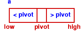Initial Step - First Partition
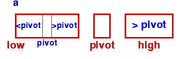	Sort Left Partition in the same way

As you can see we choose a pivot element and arrange that all the items in the lower part are less than the pivot and all those in the upper part greater than it. In the most general case, we don't know anything about the items to be sorted, so that any choice of the pivot element will do - the first element is a convenient one.

As an illustration of this idea, you can view this animation, which shows a partition algorithm in which items to be sorted are copied from the original array to a new one: items smaller than the pivot are placed to the left of the new array and items greater than the pivot are placed on the right. In the final step, the pivot is dropped into the remaining slot in the middle.

Talks:

• Three Beautiful Quicksorts by Jon Bently (Google Tech Talks August 9, 2007)

Animations

• Interactive Quicksort 1.1
• Animated Sorting Algorithms: Quicksort
• Quicksort Animation

Presentations

• QuickSort

Old News ;-)

[Apr 10, 2009] Quicksort - C++, Java, Algorithm and Data Structure Tutorials by Denis Kulagin

Contains Java and C++ implementation...

Recommended books

1. Cormen, Leiserson, Rivest. Introduction to algorithms. (Theory)
2. Aho, Ullman, Hopcroft. Data Structures and Algorithms. (Theory)
3. Robert Lafore. Data Structures and Algorithms in Java. (Practice)
4. Mark Allen Weiss. Data Structures and Problem Solving Using C++. (Practice)

Visualizers

1. Quicksort Animation (with source code line by line visualization)
2. Quicksort in Java Applets Centre
3. Animated Sorting Algorithms: Quicksort

ICS 161: Design and Analysis of Algorithms. Lecture notes for January 18, 1996

Today we'll finish heapsort, and describe both mergesort and quicksort. Why do we need multiple sorting algorithms? Different methods work better in different applications.

• Heapsort uses close to the right number of comparisons but needs to move data around quite a bit. It can be done in a way that uses very little extra memory. It's pobably good when memory is tight, and you are sorting many small items that come stored in an array.
• Merge sort is good for data that's too big to have in memory at once, because its pattern of storage access is very regular. It also uses even fewer comparisons than heapsort, and is especially suited for data stored as linked lists.
• Quicksort also uses few comparisons (somewhat more than the other two). Like heapsort it can sort "in place" by moving data in an array.

Recommended Links

Quicksort - Wikipedia, the free encyclopedia

Quicksort -- from Wolfram MathWorld

[PDF] QUICKSORT IS OPTIMAL Robert Sedgewick Jon  the quicksort cheerleader paper. Very questionable argumentation.  Optimal on what? On random data ?

NIST: balanced quicksort

Definition: A variant of quicksort which attempts to choose a pivot likely to represent the middle of the values to be sorted.

See also median.

Note: This is one of several attempts to prevent bad worst cases in quicksort by choosing the initial pivot.

Author: ASK

QuickSort Algorithm

Lecture 5 - quicksort

Analysis of Quicksort (6) Michael L. Littman; September 15th, 1998

• PROBLEM WITH QUICKSORT
  • Review
  • Quicksort Algorithm
  • Partition
  • Analysis
  • Expected Case?
  • Rock, Paper, Scissors
  • Importance of Being Random
  • Preview
• PROBABILITY THEORY
  • Probability
  • Language of Probability
  • Axioms of Probability
  • Probability Properties
  • Counting
  • Combinatorial Sample Spaces
  • Coin-flip Experiment
  • Expectation
  • Expected Running Time
  • Example
• RANDOMIZED QUICKSORT
  • Basic Idea
  • Code
  • Expected-Case Recurrence
  • Good and Bad Splits
  • Expected Run Time
  • Asymptotic Bound
  • Wrap Up

Sorting by divide-and-conquer

NIST quicksort ;www.nist.gov/dads/HTML/quicksort.html

Science Fair Projects - Quicksort

Quicksort is a well-known sorting algorithm developed by C. A. R. Hoare that, on average, needs Θ(n log n) comparisons to sort n items, while requiring Θ(n²) comparisons in the worst-case.

Quicksort's inner loop is such that it is usually easy to implement very efficiently on most computer architectures, which makes it significantly faster in practice than other Θ(n log n) algorithms that can sort in place or nearly so in the average case (recursively-implemented quicksort is not, as is sometimes regarded, an in-place algorithm, requiring Θ(log n) on average, and Θ(n) in the worst case, of stack space for recursion.)

Quicksort

Quicksort. Quicksort is a sorting algorithm that, on average, needs O(n log(n))
comparisons to sort n items. ... Quicksort was developed by CAR Hoare

[PDF] Microsoft PowerPoint - QuickSort

Quicksort Quicksort is one of the fastest and simplest sorting algorithms [Hoar]. It works recursively by a divide-and-conquer strategy

The Code Project - A QuickSort Algorithm With Customizable Swapping - C# Programming

Interactive Quicksort 1.1

Interactive Quicksort. Press "Start" to restart the algorithm. When you press the
"Start" button the algorithm will sort the numbers in the textfields. ...

Quicksort - C++, Java, Algorithm and Data Structure Tutorials by Denis Kulagin