|
|
Home | Switchboard | Unix Administration | Red Hat | TCP/IP Networks | Neoliberalism | Toxic Managers |
| (slightly skeptical) Educational society promoting "Back to basics" movement against IT overcomplexity and bastardization of classic Unix | |||||||
| See Also | Recommended Books | Recommended Links | Lecture Notes and E-books | Donald Knuth | TAOCP Volume3 | Animations | |
| Linear Search | Binary Search | Hashing | Trees | AVL trees | Fibonacci search | Humor | Etc |
|
|
Searching algorithms are closely related to the concept of dictionaries. Dictionaries are data structures that support search, insert, and delete operations. One of the most effective representations is a hash table. Typically, a simple function is applied to the key to determine its place in the dictionary. Another efficient search algorithms on sorted tables is binary search.
|
|
If the dictionary is not sorted, then heuristic methods of dynamic reorganization of the dictionary are of great value. One of the simplest are cache-based methods: several recently used keys are stored a special data structure that permits fast search (for example, located at the top and/or always sorted). Keeping the last N recently found values at the top of the table (or list) dramatically improves performance as most real life searches are cluster: if there was a request for item X[i] there is high probability that the same request will happen again after less then N lookups for other items. In the simplest form the cache can be merged with the dictionary:
move-to-front method A heuristic that moves the target of a search to the head of a list so it is found faster next time.
transposition method Search an array or list by checking items one at a time. If the value is found, swap it with its predecessor, so it is found faster next time.
In the paper
On self-organizing sequential search heuristics, Communications of the ACM, v.19
n.2, p.63-67, Feb. 1976 , R.L. Rivest presents an interesting generalization
of both methods mentioned above. The method A
You can also keep small number of "front" elements sorted and use binary search to find the element if this sorted subarray and only then linear search for the rest of array.
Among classic searching algorithms are liner search, hash tables and binary search. They can be executed on large number of various data structures such as arrays, lists, linked lists, trees.
The latter views the elements as vertices of a tree, and traverse that tree in some special order. They are often used in searching large tables on directory names in filesystems. Binary search algorithms also can be viewed as implicit tree search algorithm. Volume 3 of Knuth The Art of Computer Programming [1998] contains excellent discussions on hashing. Brief description of those algorithms can be found in Wikipedia and various electronic book, for example Sorting and Searching Algorithms: A Cookbook by Thomas Niemann.
MIT Open Courseware in Electrical Engineering and Computer Science has the following lecture Video: Lecture 9: Binary Search, Bubble and Selection Sorts by Eric Grimson and John Guttag. There is large number of useful animations of classic search algorithms. See for example Java Applets Centre
Search Algorithms Trees and Graphs
String searching algorithms are an important subdivision of search algorithms. A good description of the problem area given by Alison Cawsey (alison-ds98):
Motivation
As mentioned above, string searching algorithms are important in all sorts of applications that we meet everyday. In text editors, we might want to search through a very large document (say, a million characters) for the occurence of a given string (maybe dozens of characters). In text retrieval tools, we might potentially want to search through thousands of such documents (though normally these files would be indexed, making this unnecessary). Other applications might require string matching algorithms as part of a more complex algorithm (e.g., the Unix program ``diff'' that works out the differences between two simiar text files).
Sometimes we might want to search in binary strings (ie, sequences of 0s and 1s). For example the ``pbm'' graphics format is based on sequences of 1s and 0s. We could express a task like ``find a wide white stripe in the image'' as a string searching problem.
In all these applications the naive algorithm (that you might first think of) is rather inefficient. There are algorithms that are only a little more complex which give a very substantial increase in efficiency. In this section we'll first introduce the naive algorithm, then two increasingly sophisticated algorithms that give gains in efficiency. We'll end up discussing how properties of your string searching problem might influence choice of algorithm and average case efficiency, and how you might avoid having to search at all!
The simplest algorithm can be written in a few lines:
Procedure NaiveSearch(s1, s2: String): Integer;
{Returns an index of S2, corresponding to first match of S1 with S2, or}
{ -1 if there is no match}
var i, j: integer;
match: boolean;
begin
   i:=1; match := FALSE;
   while match = FALSE and i <= length(s1) do
     begin
       j := 1;
       {Try matching from start to end of s2, quitting when no match}
       while GetChar(s1, i) = GetChar(s2, j) and (j <= length(s2)) do
          begin
           j := j+1;           {Increment both pointers while it matches}
           i := i+1
          end;
       match := j>length(s2);       {There's a match if you got to the end of s2}
       i:= i-j+2                    {move the pointer to the first string back to
                                    {just after where you left off}
     end;
   if match
      then NaiveSearch := i-1       {If it's a match, return index of S1}
                                    {corresponding to start of match
      else NaiveSearch := -1
end;
We'll illustrate the algorithms by considering a search of string 'abc' (s2) in document 'ababcab' (s1). The following diagram should be fairly self-explanatory (the îndicates where the matching characters are checked each round):
'ababcab'               i=1,j=1
'abc'
 ^                      matches: increment i and j

'ababcab'               i=2.j=2
'abc'
  ^                     matches: increment i and j

'ababcab'               i=3,j=3
'abc'
   ^                    match fails: exit inner loop, i=i-j+2

'ababcab'               i=2, j=1
 'abc'                  match fails, exit inner loop, i=i-j+2
  ^

'ababcab'               i=3, j=1
  'abc'                 matches: increment i and j
   ^

'ababcab'               i=4, j=2
  'abc'                 matches: increment i and j
    ^

'ababcab'               i=5, j=3
  'abc'                 matches: increment i and j
     ^

                        i=6, j=4, exit loop (j>length(s2)),
                        i = 4, match=TRUE,
                        NaiveSearch = 3
Note that for this example 7 comparisons were required before the match was found. In general, if we have a string s1 or length N, s2 of length M then a maximum of approx (M-1)*N matches may be required, though often the number required will be closer to N (if few partial matches occur). To illustrate these extremes consider: s1= 'aaaabaaaabaaaaab', s2 = 'aaaaa', and s1= 'abcdefghi', s2= 'fgh'.
The Knuth-Morris-Pratt Algorithm
[Note: In this discussion I assume that we the index 1 indicates the first character in the string. Other texts may assume that 0 indicates the first character, in which case all the numbers in the examples will be one less].
The Knuth-Morris-Pratt (KMP) algorithm uses information about the characters in the string you're looking for to determine how much to `move along' that string after a mismatch occurs. To illustrate this, consider one of the examples above: s1= 'aaaabaaaabaaaaab', s2 = 'aaaaa'. Using the naive algorithm you would start off something like this:
'aaaabaaaabaaaaab'
'aaaaa'
 ^

'aaaabaaaabaaaaab'
'aaaaa'
  ^

'aaaabaaaabaaaaab'
'aaaaa'
   ^

'aaaabaaaabaaaaab'
'aaaaa'
    ^

'aaaabaaaabaaaaab'
'aaaaa'
     ^                  match fails, move s2 up one..

'aaaabaaaabaaaaab'
 'aaaaa'
  ^

etc etc
but in fact if we look at s2 (and the 'b' in s1 that caused the bad match) we can tell that there is no chance that a match starting at position 2 will work. The 'b' will end up being matched against the 4th character in s2, which is an 'a'. Based on our knowledge of s2, what we really want is the last iteration above replaced with:
'aaaabaaaabaaaaab'
     'aaaaa'
      ^
We can implement this idea quite efficiently by associating with each element position in the searched for string the amount that you can safely move that string forward if you get a mismatch in that element position. For the above example..
a 1     If mismatch in first el, just move string on 1 place.
a 2     If mismatch here, no point in trying just one place, as
        that'll involve matching with the same el (a) so move 2 places
a 3
a 4
a 5
In fact the KMP algorithm is a little more cunning than this. Consider the following case:
'aaaab'   i=3,j=3
'aab'
   ^
We can only move the second string up 1, but we KNOW that the first character will then match, as the first two elements are identical, so we want the next iteration to be:
'aaaab'  i=3,j=2
 'aab'
   ^
Note that i has not changed. It turns out that we can make things work by never decrementing i (ie, just moving forward along s1), but, given a mismatch, just decrementing j by the appropriate amount, to capture the fact that we are moving s2 up a bit along s1, so the position on s2 corresponding to i's position is lower. We can have an array giving, for each position in s2, the position in s2 that you should backup to in s2 given a mismatch (while holding the position in s1 constant). We'll call this array next[j].
j       s2[j]   next[j]
1       a       0
2       b       1
3       a       1
4       b       2
5       b       3
6       a       1
7       a       2
In fact next[1] is treated as a special case. In fact, if the first match fails we want to keep j fixed and increment i. One way to do this is to let next[1] = 0, and then have a special case that says if j=0 then increment i and j.
'abababbaa'      i=5, j=5
'ababbaa'
     ^          mismatch, so j = next[j]=3

'abababbaa'      i=5, j=3
  'ababbaa'
     ^
-------------------
'abaabbaa'      i=4, j=4
'ababbaa'
    ^           mismatch, so j = next[j]= 2

'abaababbaa'      i=5, j=2
  'ababbaa'
    ^
-------------------
'bababbaa'      i=1, j=1
'ababbaa'
 ^              mismatch, so j = next[j]= 0, increment i and j.

'abaababbaa'      i=2, j=1
 'ababbaa'
  ^
It's easy enough to implement this algorithm once you have the next[..] array. The bit that is mildly more tricky is how to calculate next[..] given a string. We can do this by trying to match a string against itself. When looking for next[j] we'd find the first index k such that s2[1..k-1] = s2[j-k+1..j-1], e.g:
'ababbaa'      s2[1..2] = s2[3..4]
  'aba....'    so next[5] = 2.
     ^
(Essentially we find next[j] by sliding forward the pattern along itself, until we find a match of the first k-1 characters with the k-1 characters before (and not including) position j).
The detailed implementations of these algorithms are left as an exercise for the reader - it's pretty easy, so long as you get the boundary cases right and avoid out-by-one errors.
The KMP algorithm is extremely simple once we have the next table:
i := 1; j:= i;
while (i <= length(s1) and j <= length(s2)) do
begin
  if (j = 0) or (GetChar(s1,i) = GetChar(s2, j)))  then begin
     i := i+1; j:= j+1
  end
  else j := next[j]
end;
(If j = length(s2) when the loop exits we have a match and can return something appropriate, such as the index in s1 where the match starts).
Although the above algorithm is quite cunning, it doesnt help that much unless the strings you are searching involve alot of repeated patterns. It'll still require you to go all along the document (s1) to be searched in. For most text editor type applications, the average case complexity is little better than the naive algorithm (O(N), where N is the length of s1). (The worst case for the KMP is N+M comparisons - much better than naive, so it's useful in certain cases).
The Boyer-Moore algorithm is significantly better, and works by searching the target string s2 from right to left, while moving it left to right along s1. The following example illustrates the general idea:
'the caterpillar'    Match fails:
'pill'               There's no space (' ') in the search string, so move it
    ^                right along 4 places

'the caterpillar'   Match fails. There's no e either, so move along 4
    'pill'
        ^

'the caterpillar'    'l' matches, so  continue trying to match right to left
        'pill'
            ^

'the caterpillar'    Match fails. But there's an 'i' in 'pill' so move along
        'pill'       to position where the 'i's line up.
           ^
'the caterpillar'    Matches, as do all the rest..
         'pill'
             ^
This still only requires knowledge of the second string, but we require an array containing an indication, for each possible character that may occur, where it occurs in the search string and hence how much to move along. So, index['p']=1, index['i']=2, index['l'] = 4 (index the rightmost 'l' where repetitions) but index['r']=0 (let the value be 0 for all characters not in the string). When a match fails at a position i in the document, at a character C we move along the search string to a position where the current character in the document is above the index[C]th character in the string (which we know is a C), and start matching again at the right hand end of the string. (This is only done when this actually results in the string being moved right - otherwise the string is just moved up one place, and the search started again from the right hand end.)
The Boyer-Moore algorithm in fact combines this method of skipping over characters with a method similar to the KMP algorithm (useful to improve efficiency after you've partially matched a string). However, we'll just assume the simpler version that skips based on the position of a character in the search string.
It should be reasonably clear that, if it is normally the case that a given letter doesnt appear at all in the search string, then this algorithm only requires approx N/M character comparisons (N=length(s1), M=length(s2)) - a big improvement on the KMP algorithm, which still requires N. However, if this is not the case then we may need up to N+M comparisons again (with the full version of the algorithm). Fortunately, for many applications we get close to the N/M performance. If the search string is very large, then it is likely that a given character WILL appear in it, but we still get a good improvement compared with the other algorithms (approx N*2/alphabet_size if characters are randomly distributed in a string).
|
|
Switchboard | ||||
| Latest | |||||
| Past week | |||||
| Past month | |||||
Nov 21, 2019 | perlmonks.org
This code was written as a solution to the problem posed in Search for identical substrings . As best I can tell it runs about 3 million times faster than the original code.
The code reads a series of strings and searches them for the longest substring between any pair of strings. In the original problem there were 300 strings about 3K long each. A test set comprising 6 strings was used to test the code with the result given below.
Someone with Perl module creation and publication experience could wrap this up and publish it if they wish.
use strict;
use warnings;
use Time::HiRes;
use List::Util qw(min max);

my $allLCS = 1;
my $subStrSize = 8; # Determines minimum match length. Should be a power of 2
# and less than half the minimum interesting match length. The larger this value
# the faster the search runs.

if (@ARGV != 1)
    {
    print "Finds longest matching substring between any pair of test strings\n";
    print "the given file. Pairs of lines are expected with the first of a\n";
    print "pair being the string name and the second the test string.";
    exit (1);
    }

# Read in the strings
my @strings;
while ()
  {
  chomp;
  my $strName = $_;
  $_ = ;
  chomp;
  push @strings, [$strName, $_];
  }

my $lastStr = @strings - 1;
my @bestMatches = [(0, 0, 0, 0, 0)]; # Best match details
my $longest = 0; # Best match length so far (unexpanded)

my $startTime = [Time::HiRes::gettimeofday ()];

# Do the search
for (0..$lastStr)
  {
  my $curStr = $_;
  my @subStrs;
  my $source = $strings[$curStr][1];
  my $sourceName = $strings[$curStr][0];

  for (my $i = 0; $i  0;
        push @localBests, [@test] if $dm >= 0;
        $offset = $test[3] + $test[4];

        next if $test[4]  0;
        push @bestMatches, [@test];
        }
        continue {++$offset;}
      }

    next if ! $allLCS;

    if (! @localBests)
      {
      print "Didn't find LCS for $sourceName and $targetName\n";
      next;
      }

    for (@localBests)
      {
      my @curr = @$_;
      printf "%03d:%03d L[%4d] (%4d %4d)\n",
        $curr[0], $curr[1], $curr[4], $curr[2], $curr[3];
      }
    }
  }

print "Completed in " . Time::HiRes::tv_interval ($startTime) . "\n";
for (@bestMatches)
  {
  my @curr = @$_;
  printf "Best match: %s - %s. %d characters starting at %d and %d.\n",
    $strings[$curr[0]][0], $strings[$curr[1]][0], $curr[4], $curr[2], $curr[3];
  }


sub expandMatch
{
my ($index1, $index2, $str1Start, $str2Start, $matchLen) = @_;
my $maxMatch = max (0, min ($str1Start, $subStrSize + 10, $str2Start));
my $matchStr1 = substr ($strings[$index1][1], $str1Start - $maxMatch, $maxMatch);
my $matchStr2 = substr ($strings[$index2][1], $str2Start - $maxMatch, $maxMatch);

($matchStr1 ^ $matchStr2) =~ /\0*$/;
my $adj = $+[0] - $-[0];
$matchLen += $adj;
$str1Start -= $adj;
$str2Start -= $adj;

return ($index1, $index2, $str1Start, $str2Start, $matchLen);
}
Output using bioMan 's six string sample:
Completed in 0.010486 Best match: >string 1 - >string 3 . 1271 characters starting at 82 an + d 82. [download]
Dec 05, 2014 | www.youtube.comPublished on
In this video you will learn about the Knuth-Morris-Pratt (KMP) string matching algorithm, and how it can be used to find string matches super fast!
KMP Algorithm explained - YouTube
Knuth-Morris-Pratt - Pattern Matching - YouTube
Nov 15, 2017 | ics.uci.edu
ICS 161: Design and Analysis of Algorithms
Lecture notes for February 27, 1996
Knuth-Morris-Pratt string matching The problem: given a (short) pattern and a (long) text, both strings, determine whether the pattern appears somewhere in the text. Last time we saw how to do this with finite automata. This time we'll go through the Knuth - Morris - Pratt (KMP) algorithm, which can be thought of as an efficient way to build these automata. I also have some working C++ source code which might help you understand the algorithm better.First let's look at a naive solution.
suppose the text is in an array: char T[n]
and the pattern is in another array: char P[m].One simple method is just to try each possible position the pattern could appear in the text.
Naive string matching :
    for (i=0; T[i] != '\0'; i++)
    {
    for (j=0; T[i+j] != '\0' && P[j] != '\0' && T[i+j]==P[j]; j++) ;
    if (P[j] == '\0') found a match
    }
There are two nested loops; the inner one takes O(m) iterations and the outer one takes O(n) iterations so the total time is the product, O(mn). This is slow; we'd like to speed it up.In practice this works pretty well -- not usually as bad as this O(mn) worst case analysis. This is because the inner loop usually finds a mismatch quickly and move on to the next position without going through all m steps. But this method still can take O(mn) for some inputs. In one bad example, all characters in T[] are "a"s, and P[] is all "a"'s except for one "b" at the end. Then it takes m comparisons each time to discover that you don't have a match, so mn overall.
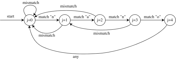
Here's a more typical example. Each row represents an iteration of the outer loop, with each character in the row representing the result of a comparison (X if the comparison was unequal). Suppose we're looking for pattern "nano" in text "banananobano".
     0  1  2  3  4  5  6  7  8  9 10 11
      T: b  a  n  a  n  a  n  o  b  a  n  o

    i=0: X
    i=1:    X
    i=2:       n  a  n  X
    i=3:          X
    i=4:             n  a  n  o
    i=5:                X
    i=6:                   n  X
    i=7:                         X
    i=8:                            X
    i=9:                               n  X
    i=10:                                 X
Some of these comparisons are wasted work! For instance, after iteration i=2, we know from the comparisons we've done that T[3]="a", so there is no point comparing it to "n" in iteration i=3. And we also know that T[4]="n", so there is no point making the same comparison in iteration i=4. Skipping outer iterations The Knuth-Morris-Pratt idea is, in this sort of situation, after you've invested a lot of work making comparisons in the inner loop of the code, you know a lot about what's in the text. Specifically, if you've found a partial match of j characters starting at position i, you know what's in positions T[i]...T[i+j-1].You can use this knowledge to save work in two ways. First, you can skip some iterations for which no match is possible. Try overlapping the partial match you've found with the new match you want to find:
    i=2: n  a  n
    i=3:    n  a  n  o
Here the two placements of the pattern conflict with each other -- we know from the i=2 iteration that T[3] and T[4] are "a" and "n", so they can't be the "n" and "a" that the i=3 iteration is looking for. We can keep skipping positions until we find one that doesn't conflict:i=2: n a n i=4: n a n oHere the two "n"'s coincide. Define the overlap of two strings x and y to be the longest word that's a suffix of x and a prefix of y. Here the overlap of "nan" and "nano" is just "n". (We don't allow the overlap to be all of x or y, so it's not "nan"). In general the value of i we want to skip to is the one corresponding to the largest overlap with the current partial match:String matching with skipped iterations :
    i=0;
    while (i<n)
    {
    for (j=0; T[i+j] != '\0' && P[j] != '\0' && T[i+j]==P[j]; j++) ;
    if (P[j] == '\0') found a match;
    i = i + max(1, j-overlap(P[0..j-1],P[0..m]));
    }
Skipping inner iterations The other optimization that can be done is to skip some iterations in the inner loop. Let's look at the same example, in which we skipped from i=2 to i=4:i=2: n a n i=4: n a n oIn this example, the "n" that overlaps has already been tested by the i=2 iteration. There's no need to test it again in the i=4 iteration. In general, if we have a nontrivial overlap with the last partial match, we can avoid testing a number of characters equal to the length of the overlap.This change produces (a version of) the KMP algorithm:
    i=0;
    o=0;
    while (i<n)
    {
    for (j=o; T[i+j] != '\0' && P[j] != '\0' && T[i+j]==P[j]; j++) ;
    if (P[j] == '\0') found a match;
    o = overlap(P[0..j-1],P[0..m]);
    i = i + max(1, j-o);
    }
The only remaining detail is how to compute the overlap function. This is a function only of j, and not of the characters in T[], so we can compute it once in a preprocessing stage before we get to this part of the algorithm. First let's see how fast this algorithm is. KMP time analysis We still have an outer loop and an inner loop, so it looks like the time might still be O(mn). But we can count it a different way to see that it's actually always less than that. The idea is that every time through the inner loop, we do one comparison T[i+j]==P[j]. We can count the total time of the algorithm by counting how many comparisons we perform.We split the comparisons into two groups: those that return true, and those that return false. If a comparison returns true, we've determined the value of T[i+j]. Then in future iterations, as long as there is a nontrivial overlap involving T[i+j], we'll skip past that overlap and not make a comparison with that position again. So each position of T[] is only involved in one true comparison, and there can be n such comparisons total. On the other hand, there is at most one false comparison per iteration of the outer loop, so there can also only be n of those. As a result we see that this part of the KMP algorithm makes at most 2n comparisons and takes time O(n).
KMP and finite automata If we look just at what happens to j during the algorithm above, it's sort of like a finite automaton. At each step j is set either to j+1 (in the inner loop, after a match) or to the overlap o (after a mismatch). At each step the value of o is just a function of j and doesn't depend on other information like the characters in T[]. So we can draw something like an automaton, with arrows connecting values of j and labeled with matches and mismatches.
The difference between this and the automata we are used to is that it has only two arrows out of each circle, instead of one per character. But we can still simulate it just like any other automaton, by placing a marker on the start state (j=0) and moving it around the arrows. Whenever we get a matching character in T[] we move on to the next character of the text. But whenever we get a mismatch we look at the same character in the next step, except for the case of a mismatch in the state j=0.
So in this example (the same as the one above) the automaton goes through the sequence of states:
    j=0
            mismatch T[0] != "n"
    j=0
            mismatch T[1] != "n"
    j=0
            match T[2] == "n"
    j=1
            match T[3] == "a"
    j=2
            match T[4] == "n"
    j=3
            mismatch T[5] != "o"
    j=1
            match T[5] == "a"
    j=2
            match T[6] == "n"
    j=3
            match T[7] == "o"
    j=4
            found match
    j=0
            mismatch T[8] != "n"
    j=0
            mismatch T[9] != "n"
    j=0
            match T[10] == "n"
    j=1
            mismatch T[11] != "a"
    j=0
            mismatch T[11] != "n"
This is essentially the same sequence of comparisons done by the KMP pseudocode above. So this automaton provides an equivalent definition of the KMP algorithm.As one student pointed out in lecture, the one transition in this automaton that may not be clear is the one from j=4 to j=0. In general, there should be a transition from j=m to some smaller value of j, which should happen on any character (there are no more matches to test before making this transition). If we want to find all occurrences of the pattern, we should be able to find an occurrence even if it overlaps another one. So for instance if the pattern were "nana", we should find both occurrences of it in the text "nanana". So the transition from j=m should go to the next longest position that can match, which is simply j=overlap(pattern,pattern). In this case overlap("nano","nano") is empty (all suffixes of "nano" use the letter "o", and no prefix does) so we go to j=0.
Alternate version of KMP The automaton above can be translated back into pseudo-code, looking a little different from the pseudo-code we saw before but performing the same comparisons.KMP, version 2 :
    j = 0;
    for (i = 0; i < n; i++)
    for (;;) {      // loop until break
        if (T[i] == P[j]) { // matches?
        j++;        // yes, move on to next state
        if (j == m) {   // maybe that was the last state
            found a match;
            j = overlap[j];
        }
        break;
        } else if (j == 0) break;   // no match in state j=0, give up
        else j = overlap[j];    // try shorter partial match
    }
The code inside each iteration of the outer loop is essentially the same as the function match from the C++ implementation I've made available. One advantage of this version of the code is that it tests characters one by one, rather than performing random access in the T[] array, so (as in the implementation) it can be made to work for stream-based input rather than having to read the whole text into memory first.The overlap[j] array stores the values of overlap(pattern[0..j-1],pattern), which we still need to show how to compute.
Since this algorithm performs the same comparisons as the other version of KMP, it takes the same amount of time, O(n). One way of proving this bound directly is to note, first, that there is one true comparison (in which T[i]==P[j]) per iteration of the outer loop, since we break out of the inner loop when this happens. So there are n of these total. Each of these comparisons results in increasing j by one. Each iteration of the inner loop in which we don't break out of the loop results in executing the statement j=overlap[j], which decreases j. Since j can only decrease as many times as it's increased, the total number of times this happens is also O(n).
Computing the overlap function Recall that we defined the overlap of two strings x and y to be the longest word that's a suffix of x and a prefix of y. The missing component of the KMP algorithm is a computation of this overlap function: we need to know overlap(P[0..j-1],P) for each value of j>0. Once we've computed these values we can store them in an array and look them up when we need them.To compute these overlap functions, we need to know for strings x and y not just the longest word that's a suffix of x and a prefix of y, but all such words. The key fact to notice here is that if w is a suffix of x and a prefix of y, and it's not the longest such word, then it's also a suffix of overlap(x,y). (This follows simply from the fact that it's a suffix of x that is shorter than overlap(x,y) itself.) So we can list all words that are suffixes of x and prefixes of y by the following loop:
    while (x != empty) {
    x = overlap(x,y);
    output x;
    }
Now let's make another definition: say that shorten(x) is the prefix of x with one fewer character. The next simple observation to make is that shorten(overlap(x,y)) is still a prefix of y, but is also a suffix of shorten(x).So we can find overlap(x,y) by adding one more character to some word that's a suffix of shorten(x) and a prefix of y. We can just find all such words using the loop above, and return the first one for which adding one more character produces a valid overlap:
Overlap computation :
    z = overlap(shorten(x),y)
    while (last char of x != y[length(z)])
    {
    if (z = empty) return overlap(x,y) = empty
    else z = overlap(z,y)
    }
    return overlap(x,y) = z
So this gives us a recursive algorithm for computing the overlap function in general. If we apply this algorithm for x=some prefix of the pattern, and y=the pattern itself, we see that all recursive calls have similar arguments. So if we store each value as we compute it, we can look it up instead of computing it again. (This simple idea of storing results instead of recomputing them is known as dynamic programming ; we discussed it somewhat in the first lecture and will see it in more detail next time .)So replacing x by P[0..j-1] and y by P[0..m-1] in the pseudocode above and replacing recursive calls by lookups of previously computed values gives us a routine for the problem we're trying to solve, of computing these particular overlap values. The following pseudocode is taken (with some names changed) from the initialization code of the C++ implementation I've made available. The value in overlap[0] is just a flag to make the rest of the loop simpler. The code inside the for loop is the part that computes each overlap value.
KMP overlap computation :
    overlap[0] = -1;
    for (int i = 0; pattern[i] != '\0'; i++) {
    overlap[i + 1] = overlap[i] + 1;
    while (overlap[i + 1] > 0 &&
           pattern[i] != pattern[overlap[i + 1] - 1])
        overlap[i + 1] = overlap[overlap[i + 1] - 1] + 1;
    }
    return overlap;
Let's finish by analyzing the time taken by this part of the KMP algorithm. The outer loop executes m times. Each iteration of the inner loop decreases the value of the formula overlap[i+1], and this formula's value only increases by one when we move from one iteration of the outer loop to the next. Since the number of decreases is at most the number of increases, the inner loop also has at most m iterations, and the total time for the algorithm is O(m).The entire KMP algorithm consists of this overlap computation followed by the main part of the algorithm in which we scan the text (using the overlap values to speed up the scan). The first part takes O(m) and the second part takes O(n) time, so the total time is O(m+n).
Nov 15, 2017 | ics.uci.edu
ICS 161: Design and Analysis of Algorithms
Lecture notes for February 27, 1996
Knuth-Morris-Pratt string matching The problem: given a (short) pattern and a (long) text, both strings, determine whether the pattern appears somewhere in the text. Last time we saw how to do this with finite automata. This time we'll go through the Knuth - Morris - Pratt (KMP) algorithm, which can be thought of as an efficient way to build these automata. I also have some working C++ source code which might help you understand the algorithm better.First let's look at a naive solution.
suppose the text is in an array: char T[n]
and the pattern is in another array: char P[m].One simple method is just to try each possible position the pattern could appear in the text.
Naive string matching :
    for (i=0; T[i] != '\0'; i++)
    {
    for (j=0; T[i+j] != '\0' && P[j] != '\0' && T[i+j]==P[j]; j++) ;
    if (P[j] == '\0') found a match
    }
There are two nested loops; the inner one takes O(m) iterations and the outer one takes O(n) iterations so the total time is the product, O(mn). This is slow; we'd like to speed it up.In practice this works pretty well -- not usually as bad as this O(mn) worst case analysis. This is because the inner loop usually finds a mismatch quickly and move on to the next position without going through all m steps. But this method still can take O(mn) for some inputs. In one bad example, all characters in T[] are "a"s, and P[] is all "a"'s except for one "b" at the end. Then it takes m comparisons each time to discover that you don't have a match, so mn overall.
Here's a more typical example. Each row represents an iteration of the outer loop, with each character in the row representing the result of a comparison (X if the comparison was unequal). Suppose we're looking for pattern "nano" in text "banananobano".
     0  1  2  3  4  5  6  7  8  9 10 11
      T: b  a  n  a  n  a  n  o  b  a  n  o

    i=0: X
    i=1:    X
    i=2:       n  a  n  X
    i=3:          X
    i=4:             n  a  n  o
    i=5:                X
    i=6:                   n  X
    i=7:                         X
    i=8:                            X
    i=9:                               n  X
    i=10:                                 X
Some of these comparisons are wasted work! For instance, after iteration i=2, we know from the comparisons we've done that T[3]="a", so there is no point comparing it to "n" in iteration i=3. And we also know that T[4]="n", so there is no point making the same comparison in iteration i=4. Skipping outer iterations The Knuth-Morris-Pratt idea is, in this sort of situation, after you've invested a lot of work making comparisons in the inner loop of the code, you know a lot about what's in the text. Specifically, if you've found a partial match of j characters starting at position i, you know what's in positions T[i]...T[i+j-1].You can use this knowledge to save work in two ways. First, you can skip some iterations for which no match is possible. Try overlapping the partial match you've found with the new match you want to find:
    i=2: n  a  n
    i=3:    n  a  n  o
Here the two placements of the pattern conflict with each other -- we know from the i=2 iteration that T[3] and T[4] are "a" and "n", so they can't be the "n" and "a" that the i=3 iteration is looking for. We can keep skipping positions until we find one that doesn't conflict:i=2: n a n i=4: n a n oHere the two "n"'s coincide. Define the overlap of two strings x and y to be the longest word that's a suffix of x and a prefix of y. Here the overlap of "nan" and "nano" is just "n". (We don't allow the overlap to be all of x or y, so it's not "nan"). In general the value of i we want to skip to is the one corresponding to the largest overlap with the current partial match:String matching with skipped iterations :
    i=0;
    while (i<n)
    {
    for (j=0; T[i+j] != '\0' && P[j] != '\0' && T[i+j]==P[j]; j++) ;
    if (P[j] == '\0') found a match;
    i = i + max(1, j-overlap(P[0..j-1],P[0..m]));
    }
Skipping inner iterations The other optimization that can be done is to skip some iterations in the inner loop. Let's look at the same example, in which we skipped from i=2 to i=4:i=2: n a n i=4: n a n oIn this example, the "n" that overlaps has already been tested by the i=2 iteration. There's no need to test it again in the i=4 iteration. In general, if we have a nontrivial overlap with the last partial match, we can avoid testing a number of characters equal to the length of the overlap.This change produces (a version of) the KMP algorithm:
    i=0;
    o=0;
    while (i<n)
    {
    for (j=o; T[i+j] != '\0' && P[j] != '\0' && T[i+j]==P[j]; j++) ;
    if (P[j] == '\0') found a match;
    o = overlap(P[0..j-1],P[0..m]);
    i = i + max(1, j-o);
    }
The only remaining detail is how to compute the overlap function. This is a function only of j, and not of the characters in T[], so we can compute it once in a preprocessing stage before we get to this part of the algorithm. First let's see how fast this algorithm is. KMP time analysis We still have an outer loop and an inner loop, so it looks like the time might still be O(mn). But we can count it a different way to see that it's actually always less than that. The idea is that every time through the inner loop, we do one comparison T[i+j]==P[j]. We can count the total time of the algorithm by counting how many comparisons we perform.We split the comparisons into two groups: those that return true, and those that return false. If a comparison returns true, we've determined the value of T[i+j]. Then in future iterations, as long as there is a nontrivial overlap involving T[i+j], we'll skip past that overlap and not make a comparison with that position again. So each position of T[] is only involved in one true comparison, and there can be n such comparisons total. On the other hand, there is at most one false comparison per iteration of the outer loop, so there can also only be n of those. As a result we see that this part of the KMP algorithm makes at most 2n comparisons and takes time O(n).
KMP and finite automata If we look just at what happens to j during the algorithm above, it's sort of like a finite automaton. At each step j is set either to j+1 (in the inner loop, after a match) or to the overlap o (after a mismatch). At each step the value of o is just a function of j and doesn't depend on other information like the characters in T[]. So we can draw something like an automaton, with arrows connecting values of j and labeled with matches and mismatches.
The difference between this and the automata we are used to is that it has only two arrows out of each circle, instead of one per character. But we can still simulate it just like any other automaton, by placing a marker on the start state (j=0) and moving it around the arrows. Whenever we get a matching character in T[] we move on to the next character of the text. But whenever we get a mismatch we look at the same character in the next step, except for the case of a mismatch in the state j=0.
So in this example (the same as the one above) the automaton goes through the sequence of states:
    j=0
            mismatch T[0] != "n"
    j=0
            mismatch T[1] != "n"
    j=0
            match T[2] == "n"
    j=1
            match T[3] == "a"
    j=2
            match T[4] == "n"
    j=3
            mismatch T[5] != "o"
    j=1
            match T[5] == "a"
    j=2
            match T[6] == "n"
    j=3
            match T[7] == "o"
    j=4
            found match
    j=0
            mismatch T[8] != "n"
    j=0
            mismatch T[9] != "n"
    j=0
            match T[10] == "n"
    j=1
            mismatch T[11] != "a"
    j=0
            mismatch T[11] != "n"
This is essentially the same sequence of comparisons done by the KMP pseudocode above. So this automaton provides an equivalent definition of the KMP algorithm.As one student pointed out in lecture, the one transition in this automaton that may not be clear is the one from j=4 to j=0. In general, there should be a transition from j=m to some smaller value of j, which should happen on any character (there are no more matches to test before making this transition). If we want to find all occurrences of the pattern, we should be able to find an occurrence even if it overlaps another one. So for instance if the pattern were "nana", we should find both occurrences of it in the text "nanana". So the transition from j=m should go to the next longest position that can match, which is simply j=overlap(pattern,pattern). In this case overlap("nano","nano") is empty (all suffixes of "nano" use the letter "o", and no prefix does) so we go to j=0.
Alternate version of KMP The automaton above can be translated back into pseudo-code, looking a little different from the pseudo-code we saw before but performing the same comparisons.KMP, version 2 :
    j = 0;
    for (i = 0; i < n; i++)
    for (;;) {      // loop until break
        if (T[i] == P[j]) { // matches?
        j++;        // yes, move on to next state
        if (j == m) {   // maybe that was the last state
            found a match;
            j = overlap[j];
        }
        break;
        } else if (j == 0) break;   // no match in state j=0, give up
        else j = overlap[j];    // try shorter partial match
    }
The code inside each iteration of the outer loop is essentially the same as the function match from the C++ implementation I've made available. One advantage of this version of the code is that it tests characters one by one, rather than performing random access in the T[] array, so (as in the implementation) it can be made to work for stream-based input rather than having to read the whole text into memory first.The overlap[j] array stores the values of overlap(pattern[0..j-1],pattern), which we still need to show how to compute.
Since this algorithm performs the same comparisons as the other version of KMP, it takes the same amount of time, O(n). One way of proving this bound directly is to note, first, that there is one true comparison (in which T[i]==P[j]) per iteration of the outer loop, since we break out of the inner loop when this happens. So there are n of these total. Each of these comparisons results in increasing j by one. Each iteration of the inner loop in which we don't break out of the loop results in executing the statement j=overlap[j], which decreases j. Since j can only decrease as many times as it's increased, the total number of times this happens is also O(n).
Computing the overlap function Recall that we defined the overlap of two strings x and y to be the longest word that's a suffix of x and a prefix of y. The missing component of the KMP algorithm is a computation of this overlap function: we need to know overlap(P[0..j-1],P) for each value of j>0. Once we've computed these values we can store them in an array and look them up when we need them.To compute these overlap functions, we need to know for strings x and y not just the longest word that's a suffix of x and a prefix of y, but all such words. The key fact to notice here is that if w is a suffix of x and a prefix of y, and it's not the longest such word, then it's also a suffix of overlap(x,y). (This follows simply from the fact that it's a suffix of x that is shorter than overlap(x,y) itself.) So we can list all words that are suffixes of x and prefixes of y by the following loop:
    while (x != empty) {
    x = overlap(x,y);
    output x;
    }
Now let's make another definition: say that shorten(x) is the prefix of x with one fewer character. The next simple observation to make is that shorten(overlap(x,y)) is still a prefix of y, but is also a suffix of shorten(x).So we can find overlap(x,y) by adding one more character to some word that's a suffix of shorten(x) and a prefix of y. We can just find all such words using the loop above, and return the first one for which adding one more character produces a valid overlap:
Overlap computation :
    z = overlap(shorten(x),y)
    while (last char of x != y[length(z)])
    {
    if (z = empty) return overlap(x,y) = empty
    else z = overlap(z,y)
    }
    return overlap(x,y) = z
So this gives us a recursive algorithm for computing the overlap function in general. If we apply this algorithm for x=some prefix of the pattern, and y=the pattern itself, we see that all recursive calls have similar arguments. So if we store each value as we compute it, we can look it up instead of computing it again. (This simple idea of storing results instead of recomputing them is known as dynamic programming ; we discussed it somewhat in the first lecture and will see it in more detail next time .)So replacing x by P[0..j-1] and y by P[0..m-1] in the pseudocode above and replacing recursive calls by lookups of previously computed values gives us a routine for the problem we're trying to solve, of computing these particular overlap values. The following pseudocode is taken (with some names changed) from the initialization code of the C++ implementation I've made available. The value in overlap[0] is just a flag to make the rest of the loop simpler. The code inside the for loop is the part that computes each overlap value.
KMP overlap computation :
    overlap[0] = -1;
    for (int i = 0; pattern[i] != '\0'; i++) {
    overlap[i + 1] = overlap[i] + 1;
    while (overlap[i + 1] > 0 &&
           pattern[i] != pattern[overlap[i + 1] - 1])
        overlap[i + 1] = overlap[overlap[i + 1] - 1] + 1;
    }
    return overlap;
Let's finish by analyzing the time taken by this part of the KMP algorithm. The outer loop executes m times. Each iteration of the inner loop decreases the value of the formula overlap[i+1], and this formula's value only increases by one when we move from one iteration of the outer loop to the next. Since the number of decreases is at most the number of increases, the inner loop also has at most m iterations, and the total time for the algorithm is O(m).The entire KMP algorithm consists of this overlap computation followed by the main part of the algorithm in which we scan the text (using the overlap values to speed up the scan). The first part takes O(m) and the second part takes O(n) time, so the total time is O(m+n).
Published on Dec 5, 2014In this video you will learn about the Knuth-Morris-Pratt (KMP) string matching algorithm, and how it can be used to find string matches super fast!
KMP Algorithm explained - YouTube
Knuth-Morris-Pratt - Pattern Matching - YouTube
KMP Algorithm explained - YouTube
KMP Searching Algorithm - YouTube
Nov 15, 2017 | www.youtube.com
Preface
This is a collection of algorithms for sorting and searching. Descriptions are brief and intuitive, with just enough theory thrown in to make you nervous. I assume you know a high-level language, such as C, and that you are familiar with programming concepts including arrays and pointers.
The first section introduces basic data structures and notation. The next section presents several sorting algorithms. This is followed by a section on dictionaries, structures that allow efficient insert, search, and delete operations. The last section describes algorithms that sort data and implement dictionaries for very large files. Source code for each algorithm, in ANSI C, is included.
Most algorithms have also been coded in Visual Basic. If you are programming in Visual Basic, I recommend you read Visual Basic Collections and Hash Tables, for an explanation of hashing and node representation.
If you are interested in translating this document to another language, please send me email. Special thanks go to Pavel Dubner, whose numerous suggestions were much appreciated. The following files may be downloaded:
source code (C) (24k)
source code (Visual Basic) (27k)
Permission to reproduce portions of this document is given provided the web site listed below is referenced, and no additional restrictions apply. Source code, when part of a software project, may be used freely without reference to the author.
Thomas Niemann
Portland, Oregon epaperpress.com
About: C Minimal Perfect Hashing Library is a portable LGPL library to create and to work with minimal perfect hashing functions. The library encapsulates the newest and more efficient algorithms available in the literature in an easy-to-use, production-quality, fast API. The library is designed to work with big entries that cannot fit in the main memory. It has been used successfully for constructing minimal perfect hashing functions for sets with billions of keys.
Changes: This version adds the internal memory bdz algorithm and utility functions to (de)serialize minimal perfect hash functions from mmap'ed memory regions. The new bdz algorithm for minimal perfect hashes requires 2.6 bits per key and is the fastest one currently available in the literature.
This research is all concerned with the development of an analysis and simulations of the effect of mixed deletions and insertions in binary search trees. Previously it was believed that the average depth of a node in a tree subjected to updates was decreased towards an optimal O(log n) when using the usual algorithms (See e.g. Knuth Vol. 3 [8] ) This was supported to some extent by a complete analysis for trees of only three nodes by Jonassen and Knuth [7] in 1978. Eppinger [6] performed some simulations showing that this was likely false, and conjectured, based on the experimental evidence, that the depth grew as O(log^3 n), but offered no analysis or explanation as to why this should occur. Essentially, this problem concerning one of the most widely used data structures had remained open for 20 years.Both my MSc [1] and Ph.D. [2] focused on this problem. This research indicates that in fact the depth grows as O(n^{1/2}). A proof under certain simplifying assumptions was given in the theoretical analysis in Algorithmica [3], while a set of simulations was presented together with a less formal analysis of the more general case, in the Computer Journal [4] , intended for a wider audience. A complete analysis for the most general case is still open.
More recently P. Evans [5] has demonstrated that asymmetry may be even more dangerous in smaller doses! Algorithms with only occasional asymmetric moves tend to develop trees with larger skews, although the effects take much longer.
Publications
- Joseph Culberson. Updating Binary Trees. MSc Thesis, University of Waterloo Department of Computer Science, 1984. (Available as Waterloo Research Report CS-84-08.) Abstract
- Joseph Culberson. The Effect of Asymmetric Deletions on Binary Search Trees. Ph. D. Thesis University of Waterloo Department of Computer Science, May 1986. (Available as Waterloo Research Report CS-86-15.) Abstract
- Joseph Culberson J. Ian Munro. Analysis of the standard deletion algorithms in exact fit domain binary search trees. Algorithmica, vol 6, 295-311, 1990. Abstract
- Joseph Culberson J. Ian Munro. Explaining the behavior of binary search trees under prolonged updates: A model and simulations. The Computer Journal, vol 32(1), 68-75, February 1989. Abstract
- Joseph C. Culberson and Patricia A. Evans Asymmetry in Binary Search Tree Update Algorithms Technical Report TR94-09
Other References
- Jeffery L. Eppinger. An empirical study of insertion and deletion in binary trees. Communications of the ACM vol. 26, September 1983.
- Arne T. Jonassen and Donald E. Knuth A trivial algorithm whose analysis isn't. Journal of Computer and System Sciences, 16:301-322, 1978.
- D. E. Knuth Sorting and Searching Volume III, The Art of Computer Programming Addison-Wesley Publishing Company, Inc., Reading, Massachusetts, 1973.
In [3], R.L. Rivest presents a set of methods for dynamically reordering a sequential list containing N records in order to increase search efficiency. The method A
i (for i between 1 and N) performs the following operation each time that a record R has been successfully retrieved: Move R forward i positions in the list, or to the front of the list if it was in a position less than i. The method A1 is called the transposition method, and the method AN-1 is called the move-to-front method.
Google matched content |
Preface
This is a collection of algorithms for sorting and searching. Descriptions are brief and intuitive, with just enough theory thrown in to make you nervous. I assume you know a high-level language, such as C, and that you are familiar with programming concepts including arrays and pointers.
The first section introduces basic data structures and notation. The next section presents several sorting algorithms. This is followed by a section on dictionaries, structures that allow efficient insert, search, and delete operations. The last section describes algorithms that sort data and implement dictionaries for very large files. Source code for each algorithm, in ANSI C, is included.
Most algorithms have also been coded in Visual Basic. If you are programming in Visual Basic, I recommend you read Visual Basic Collections and Hash Tables, for an explanation of hashing and node representation.
If you are interested in translating this document to another language, please send me email. Special thanks go to Pavel Dubner, whose numerous suggestions were much appreciated. The following files may be downloaded:
source code (C) (24k)
source code (Visual Basic) (27k)
Permission to reproduce portions of this document is given provided the web site listed below is referenced, and no additional restrictions apply. Source code, when part of a software project, may be used freely without reference to the author.
Thomas Niemann
Portland, Oregon epaperpress.com
Linear search - encyclopedia article about Linear search.
In the previous labs we have already dealt with linear search, when we talked about lists. Linear Search in Scheme is probably the simplest example of a storage/retrieval datastructure due to the number of primitive operations on lists that we can use. For instance, creation of the datastructure just requires defining a null list.
There are two types of linear search we will examine. The first is search in an unordered list; we have seen this already in the lab about cockatoos and gorillas. All of the storage retrieval operations are almost trivial: insertion is just a single cons of the element on the front of the list. Search involves recurring down the list, each time checking whether the front of the list is the element we need. Deletion is similar to search, but we cons the elements together as we travel down the list until we find the element, at which point we return the cdr of the list. We also did analysis on these algorithms and deduced that the runtime is O(n).
C++ Examples - Linear Search in a Range
On the Competitiveness of Linear Search
C++ Notes: Algorithms: Linear Search
CSC 108H - Lecture Notes
... Linear Search (Sequential). Start with
the first name, and continue looking until
x is found. Then print corresponding phone number. ... Linear Search
(on a Vector). ...
Linear Search: 1.1 Description/Definition
The simplest of these searches is the Linear Search.
A Linear Search is simply searching
through a line of objects in order to find a particular item. ...
Linear Search
Linear Search. No JDK 1.3 support, applet not shown.
www.cs.usask.ca/.../csconcepts/2002_7/static/ tutorial/introduction/linearsearchapp/linearsearch.html - 2k -Cached - Similar pages
Move to the front (self-organizing) modification
Linear Search the Transpose Method
Here the heuristic is slightly different from the Move-To-Front method : once found, the transition is swapped with the immediately preceding one, performing an incremental bubble sort at each access.
Of course, these two techniques provide a sensitive speed-up only if the probabilities for each transition to be accessed are not uniform.
These are the seven representations that caught our attention at first but that set of containers will be broadened when a special need is to be satisfied.
What is obvious here is that each of these structures has advantages and drawbacks, whether on space complexity or on time complexity. All these constraints have to be taken in account in order to construct code adapted to particuliar situations.Linear Search : the Move-To-Front Method
Self-organizing linear search
... Self-organizing linear search. Full text, pdf formatPdf (1.73 MB). ... ABSTRACT Algorithms
that modify the order of linear search lists are surveyed. ...
portal.acm.org/citation.cfm?id=5507 - Similar pages
Definition: Search a sorted array by repeatedly dividing the search interval in half. Begin with an interval covering the whole array. If the value of the search key is less than the item in the middle of the interval, narrow the interval to the lower half. Otherwise narrow it to the upper half. Repeatedly check until the value is found or the interval is empty.
Generalization (I am a kind of ...)
dichotomic search.Aggregate parent (I am a part of or used in ...)
binary insertion sort, ideal merge, suffix array.Aggregate child (... is a part of or used in me.)
divide and conquer.See also linear search, interpolation search, Fibonaccian search, jump search.
Note: Run time is O(ln n). The search implementation in C uses 0-based indexing.
Author: PEB
Implementation
search (C) n is the highest index of the 0-based array; possible key indexes, k, are low < k <= high in the loop. (Scheme), Worst-case behavior annotated for real time (WOOP/ADA), including bibliography.
en.wikipedia.org/wiki/Binary_search
Binary Search Trees http://ciips.ee.uwa.edu.au/~morris/Year2/PLDS210/niemann/s_bin.htm
Binary Search Tree http://www.personal.kent.edu/~rmuhamma/Algorithms/MyAlgorithms/binarySearchTree.htm
(see also Libraries -- there are a several libraries that implementat AVL trees)
(see The Fibonacci Numbers and Golden section in Nature for information about Fibinacci, who introduced the decimal number system into Europe and first suggested a problem that lead to Fibonacci numbers)
Here is the method for the continuous case:
The fibonacci search method minimizes the maximum number of evaluations needed to reduce the interval of uncertainty to within the prescribed length. For example, it will reduce the length of a unit interval [0,1] to 1/10946 (= .00009136) with only 20 evaluations. In the case of a finite set, fibonacci search finds the maximum value of a unimodal function on 10,946 points with only 20 evaluations, but this can be improved -- see lattice search.
For very large N, the placement ratio (g_N) approaches the golden mean, and the method approaches the golden section search. Here is a comparison of interval reduction lengths for fibonacci, golden section and dichotomous search methods. In each case N is the number of evaluations needed to reduce length of the interval of uncertainty to 1/F_N. For example, with 20 evaluations dichotomous search reduces the interval of uncertainty to .0009765 of its original length (with separation value near 0). The most reduction comes from fibonacci search, which is more than an order of magnitude better, at .0000914. Golden section is close (and gets closer as N gets larger).
    Evaluations  Fibonacci      Dichotomous      Golden section
        N          1/F_N        1/2^|_N/2_|      1/(1.618)^(N-1)
    ============================================================
        5         .125            .25              .146
       10         .0112           .0312            .0131
       15         .00101          .00781           .00118
       20         .0000914        .000976          .000107
       25         .00000824       .0002441         .0000096
    =============================================================
Here is a biography of Fibonacci.
         N    F_N
       ==============
         0      1
         1      1
         2      2
         3      3
         4      5
         5      8
         6     13
         7     21
         8     34
         9     55
        10     89
        20  10946
        50    2.0E10
       100    5.7E20
      ==============
Named after the 13th century mathematician who discovered it, this sequence has many interesting properties, notably for an optimal univariate optimization strategy, called fibonacci search
Society
Groupthink : Two Party System as Polyarchy : Corruption of Regulators : Bureaucracies : Understanding Micromanagers and Control Freaks : Toxic Managers : Harvard Mafia : Diplomatic Communication : Surviving a Bad Performance Review : Insufficient Retirement Funds as Immanent Problem of Neoliberal Regime : PseudoScience : Who Rules America : Neoliberalism : The Iron Law of Oligarchy : Libertarian Philosophy
Quotes
War and Peace : Skeptical Finance : John Kenneth Galbraith :Talleyrand : Oscar Wilde : Otto Von Bismarck : Keynes : George Carlin : Skeptics : Propaganda : SE quotes : Language Design and Programming Quotes : Random IT-related quotes : Somerset Maugham : Marcus Aurelius : Kurt Vonnegut : Eric Hoffer : Winston Churchill : Napoleon Bonaparte : Ambrose Bierce : Bernard Shaw : Mark Twain Quotes
Bulletin:
Vol 25, No.12 (December, 2013) Rational Fools vs. Efficient Crooks The efficient markets hypothesis : Political Skeptic Bulletin, 2013 : Unemployment Bulletin, 2010 : Vol 23, No.10 (October, 2011) An observation about corporate security departments : Slightly Skeptical Euromaydan Chronicles, June 2014 : Greenspan legacy bulletin, 2008 : Vol 25, No.10 (October, 2013) Cryptolocker Trojan (Win32/Crilock.A) : Vol 25, No.08 (August, 2013) Cloud providers as intelligence collection hubs : Financial Humor Bulletin, 2010 : Inequality Bulletin, 2009 : Financial Humor Bulletin, 2008 : Copyleft Problems Bulletin, 2004 : Financial Humor Bulletin, 2011 : Energy Bulletin, 2010 : Malware Protection Bulletin, 2010 : Vol 26, No.1 (January, 2013) Object-Oriented Cult : Political Skeptic Bulletin, 2011 : Vol 23, No.11 (November, 2011) Softpanorama classification of sysadmin horror stories : Vol 25, No.05 (May, 2013) Corporate bullshit as a communication method : Vol 25, No.06 (June, 2013) A Note on the Relationship of Brooks Law and Conway Law
History:
Fifty glorious years (1950-2000): the triumph of the US computer engineering : Donald Knuth : TAoCP and its Influence of Computer Science : Richard Stallman : Linus Torvalds : Larry Wall : John K. Ousterhout : CTSS : Multix OS Unix History : Unix shell history : VI editor : History of pipes concept : Solaris : MS DOS : Programming Languages History : PL/1 : Simula 67 : C : History of GCC development : Scripting Languages : Perl history : OS History : Mail : DNS : SSH : CPU Instruction Sets : SPARC systems 1987-2006 : Norton Commander : Norton Utilities : Norton Ghost : Frontpage history : Malware Defense History : GNU Screen : OSS early history
Classic books:
The Peter Principle : Parkinson Law : 1984 : The Mythical Man-Month : How to Solve It by George Polya : The Art of Computer Programming : The Elements of Programming Style : The Unix Hater’s Handbook : The Jargon file : The True Believer : Programming Pearls : The Good Soldier Svejk : The Power Elite
Most popular humor pages:
Manifest of the Softpanorama IT Slacker Society : Ten Commandments of the IT Slackers Society : Computer Humor Collection : BSD Logo Story : The Cuckoo's Egg : IT Slang : C++ Humor : ARE YOU A BBS ADDICT? : The Perl Purity Test : Object oriented programmers of all nations : Financial Humor : Financial Humor Bulletin, 2008 : Financial Humor Bulletin, 2010 : The Most Comprehensive Collection of Editor-related Humor : Programming Language Humor : Goldman Sachs related humor : Greenspan humor : C Humor : Scripting Humor : Real Programmers Humor : Web Humor : GPL-related Humor : OFM Humor : Politically Incorrect Humor : IDS Humor : "Linux Sucks" Humor : Russian Musical Humor : Best Russian Programmer Humor : Microsoft plans to buy Catholic Church : Richard Stallman Related Humor : Admin Humor : Perl-related Humor : Linus Torvalds Related humor : PseudoScience Related Humor : Networking Humor : Shell Humor : Financial Humor Bulletin, 2011 : Financial Humor Bulletin, 2012 : Financial Humor Bulletin, 2013 : Java Humor : Software Engineering Humor : Sun Solaris Related Humor : Education Humor : IBM Humor : Assembler-related Humor : VIM Humor : Computer Viruses Humor : Bright tomorrow is rescheduled to a day after tomorrow : Classic Computer Humor
The Last but not Least Technology is dominated by two types of people: those who understand what they do not manage and those who manage what they do not understand ~Archibald Putt. Ph.D
Copyright © 1996-2021 by Softpanorama Society. www.softpanorama.org was initially created as a service to the (now defunct) UN Sustainable Development Networking Programme (SDNP) without any remuneration. This document is an industrial compilation designed and created exclusively for educational use and is distributed under the Softpanorama Content License. Original materials copyright belong to respective owners. Quotes are made for educational purposes only in compliance with the fair use doctrine.
FAIR USE NOTICE This site contains copyrighted material the use of which has not always been specifically authorized by the copyright owner. We are making such material available to advance understanding of computer science, IT technology, economic, scientific, and social issues. We believe this constitutes a 'fair use' of any such copyrighted material as provided by section 107 of the US Copyright Law according to which such material can be distributed without profit exclusively for research and educational purposes.
This is a Spartan WHYFF (We Help You For Free) site written by people for whom English is not a native language. Grammar and spelling errors should be expected. The site contain some broken links as it develops like a living tree...
|
|
You can use PayPal to to buy a cup of coffee for authors of this site |
Disclaimer:
The statements, views and opinions presented on this web page are those of the author (or referenced source) and are not endorsed by, nor do they necessarily reflect, the opinions of the Softpanorama society. We do not warrant the correctness of the information provided or its fitness for any purpose. The site uses AdSense so you need to be aware of Google privacy policy. You you do not want to be tracked by Google please disable Javascript for this site. This site is perfectly usable without Javascript.
Last modified: November 23, 2019